1. ML: Basic Fundamentals

📅 2026-01-30 | #ML

Dataset Representation

Tabular datasets consists of rows and columns :

Rows : Also called data points, samples, observations, instances, patterns.
- Each row reprsents a single observation.
Columns : Also called variables, characteristics, features, attribute.
- Each columns represents a measurable property or attribute of that observation.

	H	W
$p_{1}$	130	55
$p_{2}$	140	65
$⋮$	$⋮$	$⋮$
$p_{n}$	160	75

To perform statistical analysis, the datasets is viewed as samples drawn from a probability distribution.

Each feature (column) is treated as Random Variable ( $X$ ).
- A RV is a function that maps outcomes of a random phenomenon to numerical values.
- Thus, $X_{h e i g h t}$ is a rv describing the distribution of heights feature in the population.
A single row containing $d$ features is a random vector.
- If the dataset has features $X_{1}$ , $X_{2}$ , $\dots$ , $X_{d}$ , then a single observation is a vector $x = [x_{1}, x_{2}, \dots, x_{d}]^{T}$ .
Thus, the entire dataset is a collection of $n$ observed random vectors :

D = {x_{1}, x_{2}, \dots, x_{n}} = Dataset

x_{i} = [x_{i 1}, x_{i 2}, \dots, x_{i d}]^{T} random vector

Thus, the full table can be visualized like :

X = x_{1}^{T} x_{2}^{T} ⋮ x_{n}^{T} = x_{11} x_{21} ⋮ x_{n 1} x_{12} x_{22} ⋮ x_{n 2} \dots \dots ⋱ \dots x_{1 d} x_{2 d} ⋮ x_{n d}

Measures of Central Tendencies

Moment 1

1. Mean

μ = \frac{1}{n} i = 1 \sum n x_{i} = \overset{x}{ˉ}

For a dataset :

X = x_{11} x_{21} ⋮ \overset{x}{ˉ}_{1} x_{n 1} x_{12} x_{22} ⋮ \overset{x}{ˉ}_{2} x_{n 2} x_{13} x_{23} ⋮ \overset{x}{ˉ}_{3} x_{n 3} \dots \dots ⋱ \dots x_{1 d} x_{2 d} ⋮ \overset{x}{ˉ}_{d} x_{n d}

Where :

$\overset{x}{ˉ}_{j} = \frac{1}{n} \sum_{i = 1}^{n} x_{ij}$

And thus the resulting mean vector $μ$ is a collection of these individual feature means :

μ = \overset{ˉ}{X} = [\overset{x}{ˉ}_{1} \overset{x}{ˉ}_{2} \overset{x}{ˉ}_{3} \dots \overset{x}{ˉ}_{d}]^{T}

2. Median

First, sort the data in ascending order.

If odd no. of values :

Median = x_{\frac{n + 1}{2}}

If even no. of values :

Median = \frac{1}{2} [x_{\frac{n}{2}} + x_{\frac{n + 1}{2}}]

Red: When outliers are present in the dataset, it is better to use median.

Moment 2 (Measures of Dispersion)

3. Variance

Measures how far are data points spread out from the mean.

σ^{2} = \frac{1}{n - 1} i = 1 \sum n (x_{i} - μ)^{2}

It heavily weight the outliers because it squares the difference.

4. Standard Deviation

σ = \frac{1}{n - 1} i = 1 \sum n (x_{i} - μ)^{2}

Square root of variance.
It measures the average distance of data points from the mean.

5. Range

Range = x_{ma x} - x_{min}

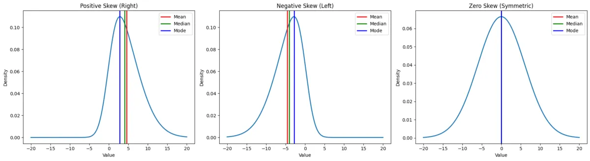
Moment 3 / Skewness

Measures the asymmetry / symmetry of the distribution around the mean.

Skewness = \frac{1}{n} \sum (\frac{x _{i} - μ}{σ})^{3}

Positive Skew : Tail extends to the right (right skewed).
Negative Skew : Tail extends to the left (left skewed).
Zero Skew : Perfectly symmetrical (like a standard Normal distribution).

Skewness

Moment 4 / Kurtosis

It defines the shape in terms of peak (sharpness) and tail (heaviness).

Kurtosis = \frac{1}{n} \sum (\frac{x _{i} - μ}{σ})^{4}

Green: In denominator, Bessels correction (use of $n - 1$ ) will be done when a sample of the population is considered. Otherwise, when the whole population is used, use $n$ .

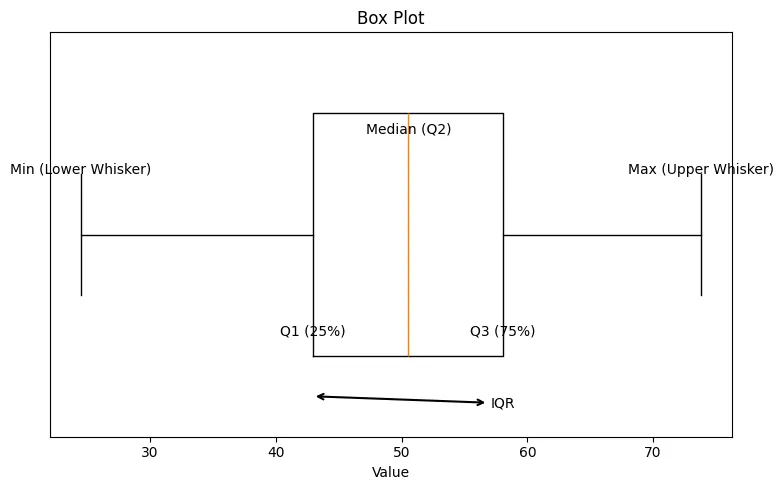
Box Plot

It is a standard way of displaying the distribution of data based on 5-number summary.

Minimum ( $Q_{0}$ ) : lowest data point excluding any outliers.
First Quartile ( $Q_{1}$ / 25th Percentile) : The value below which 25% of the data falls. The bottom of the box.
Median ( $Q_{2}$ / 50th Percentile) : The middle value of the dataset. The line inside the box.
Third Quartile ( $Q_{3}$ / 75th Percentile) : The value below which 75% of the data falls. The top of the box.
Maximum ( $Q_{4}$ ) : The highest data point excluding any outliers.

Interquartile Range (IQR) : The height of the box ( $Q_{3} - Q_{1}$ ). It represents the middle 50% of the data.
Whiskers : Lines extending from the box indicating variability outside the upper and lower quartiles.
- Set to $Q_{1} - 1.5 \times I QR$ and $Q_{3} + 1.5 \times I QR$
Outliers : Individual points plotted beyond the whiskers.

Box Plot

Covariance and Correlation

When analysing 2 features or Random Variables ( $X$ and $Y$ ), it is better to look at their joint variability.

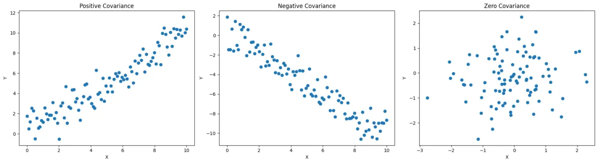
Covariance

C o v (X, Y) = \frac{1}{n - 1} \sum [(X - \overset{ˉ}{X}) (Y - \overset{ˉ}{Y})]

= E [(X - μ_{X}) (Y - μ_{Y})]

It measures the direction of the linear relationship between variables.

Positive Covariance : As $X$ increases, $Y$ tends to increase.
Negative Covariance : As $X$ increases, $Y$ tends to decrease.
Zero Covariance : No linear relationship between the 2 RVs.

Covariance

Correlation

It is the normalized version of covariance. It measures both the strength and direction of linear relationship.

ρ_{X, Y} = \frac{C o v ( X , Y )}{σ _{X} σ _{Y}}

It is the Pearson Correlation Coefficient.
It will always be between 1 and -1.

Orange: Covariance of a RV ' $X$ ' with itself will be $(E [X - E [X]) (E [X - E [X]]) = E [(X - E [X])^{2}] = σ_{X}^{2}$ .
Thus, $C o v (X, X) = Va r (X)$ .

Covariance Matrix

For a random vector with $d$ features, the relation between all features can be summarized using the Covariance Matrix $(\sum)$ .

It is a $d \times d$ matrix.

Σ = Va r (X_{1}) C o v (X_{2}, X_{1}) ⋮ C o v (X_{d}, X_{1}) C o v (X_{1}, X_{2}) Va r (X_{2}) ⋮ C o v (X_{d}, X_{2}) \dots \dots ⋱ \dots C o v (X_{1}, X_{d}) C o v (X_{2}, X_{d}) ⋮ Va r (X_{d})

Diagonal elements : Variance of individual terms.
Off-Diagonal elements : Covariances between feature pairs.
- $C o v (X, Y) = C o v (Y, X)$ , this means that the matrix is symmetric.

Green: If one feature is a perfect linear combination of other features, then there is redundancy in the information, and the covariance matrix is singular (i.e., its rank is less than the number of features).

Correlation Matrix

While the Covariance Matrix tells the direction of the relationship and the spread, the Correlation Matrix provides a normalized score of the relationship strength, making it easier to compare features with different units (e.g., comparing "Height in cm" vs. "Weight in kg").

R = 1 ρ_{21} ⋮ ρ_{d 1} ρ_{12} 1 ⋮ ρ_{d 2} \dots \dots ⋱ \dots ρ_{1 d} ρ_{2 d} ⋮ 1

$ρ_{ij}$ : It is the Pearson Coefficient.
- $ρ_{ij} = \frac{C o v ( X _{i} , X _{j} )}{σ _{X_{i}} σ _{X_{j}}}$
It is between $[1, - 1]$ .
It is also a symmetric matrix.

Types of Machine Learnings

Supervised Learning

Model learns from labelled data. For every input, the correct output is already known. The goal is for the algorithm to learn the mapping function from the input to the output.
Eg. : Linear Regression, Logistic Regression, SVM, Decision Tree, KNN, Neural Networks, etc.
Use cases : Email spam filtering, Medical diagnosis, Credit Scoring, etc.

Unsupervised Learning

The model works with unlabelled data and finds hidden patterns.
Eg. Clustering, Dimensionality Reduction (PCA)
Use cases : Customer segmentation, Anomaly detection, Association discovery

Semi-Supervised Learning

The model is trained on a small amount of labeled data and a large amount of unlabeled data.
eg. Self-training models, Transformers
Image classification when labelling data is expensive.

Reinforcement Learning

An agent learns to make decisions by performing actions in an environment to achieve a goal. It receives rewards for good actions and penalties for bad ones.
Examples : Policy Gradient Methods
Use cases : Robotics, Self-driving cars, Game plating (chess, go)

Supervised Learning

Start with a labelled dataset where input (features) and outputs (labels) are known.
Split the dataset into train-test.

Training Set : Used to build and tune models.
- It is split into 2 parts :
  - Train split
  - Validation split
Test Set : Held out and never used during training or model selection. It is only used at the very end to estimate real-world performance.

Using the training set, multiple candidate models are fitted based on different hyperparameters or algos.
Validation set is used to evaluate these models during development.
Based on the validation performance the best model is selected (highest validation accuracy, lowest loss).
The selected model becomes the final trained model.
It is evaluated on the test set, producing an unbiased estimate of the performance.

With this, the basics are over.