4. ML: Confusion Matrix, Bias-Variance & Regularization
#Model Evaluation : Confusion Matrix & Metrics
To optimize a model, its performance must be defined. In classification, raw accuracy is often insufficient, especially with imbalanced classes. The foundation of evaluation is the Confusion Matrix.
For a binary classifier, the predictions are categorized into 4 buckets based on the intersection of the predicted class and the actual truth values.
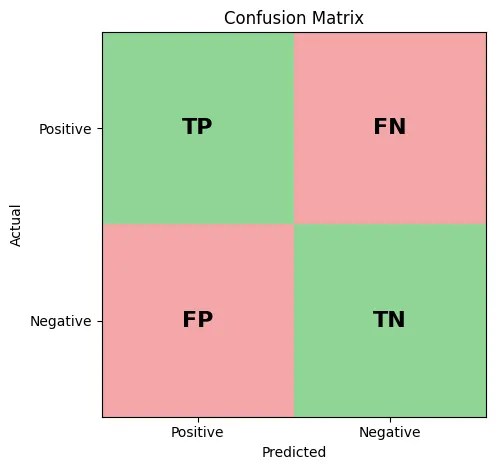
Confusion Matrix
- True Positive (TP): Predicted (+) and Actual (+).
- True Negative (TN): Predicted (-) and Actual (-).
- False Positive (FP): Predicted (+) and Actual (-) (Type I Error).
- False Negative (FN): Predicted (-) and Actual (+) (Type II Error).
These 4 values are used to derive metrics to evaluate specific aspects of the model performance :
#1. Accuracy
Ratio of correct prediction to the total pool.
- Accuracy fails to distinguish between types of errors which is critical in unbalanced datasets.
#2. Precision
The percentage of predicted positives that are actually positive.
- High precision means low False Positives.
- Positive Predictive Value
#3. Recall
The percentage of actual positives that were correctly identified.
- Sensitivity/True Positive Rate
- High recall means low False Negatives.
#4. Selectivity (Specificity) :
While Recall measures how well we find positives, Selectivity measures how well we reject negatives.
#5. F1-Score
The harmonic mean of Precision and Recall.
- It penalizes extreme values more than the arithmetic mean, ensuring a model is balanced.
#6. Area Under ROC Curve (AUC-ROC)
ROC Curve Definition
The Receiver Operating Characteristic (ROC) curve plots the Recall (TPR) against the False Positive Rate at various threshold settings.
The Area Under this Curve (AUC) represents the probability that the classifier will rank a randomly chosen positive instance higher than a randomly chosen negative one.
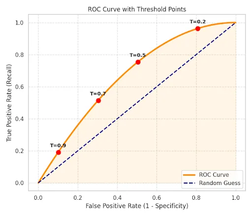
AUC-ROC
In case of more than 2 classes, compute Precision/Recall for each class independently, then average the scores. Treats all classes equally (good for checking performance on rare classes).
#Bias-Variance Trade-Off
One of the most fundamental problem is Generalization : Creating a hypothesis that performs well on unseen data.
The error of a model can be decomposed into 3 parts : Bias, Variance & Irreducible Error.
#Bias
It is the error caused by oversimplifying assumptions in the model. A high bias model will be too simple for the model and miss important patterns in the data. It will lead to underfitting.
Bias measures how far the average prediction of a model (over many different training sets) is from the true function.
#Variance
Variance is error caused by too much sensitivity to the training data. A high variance model will be too complex and fit the noise in the training data. It will lead to overfitting.
Variance measures how much the model’s predictions would change if it were trained on a different dataset.

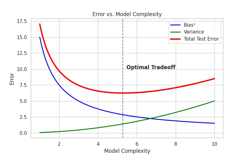
Bias-Variance
#Mathematical Derivation of MSE Decomposition
Assume a true relationship , where is noise. We estimate this with a model .
The expected mean squared error (MSE) on an unseen sample is:
Focusing on the estimation error ,
Let be the average prediction of our model over infinite training sets. We add and subtract this term :
Expanding this square :
- Bias term : is the squared Bias.
- It measures how far the average model is from the truth.
- Variance term : is the Variance.
- It measures how much any single model fluctuates around the average model.
- Cross term : The cross term vanishes because .
Thus the Final Relation
Thus, the error is made up of bias and variance and it is important to find the right balance.
- Low Complexity : High Bias, Low Variance. The model is too rigid.
- High Complexity : Low Bias, High Variance. The model is too flexible and captures noise.
- The Sweet Spot : The goal is to find the complexity level where the sum of Bias and Variance is minimized.
Bias-Variance Tradeoff
- Underfitting : Occurs when a model is too simple to capture underlying patterns, performing poorly on both training and test data.
- Overfitting : Occurs when a model is too complex and learns noise in the training data as if it were a real pattern. It leads to high accuracy on training data but poor performance on testing data.
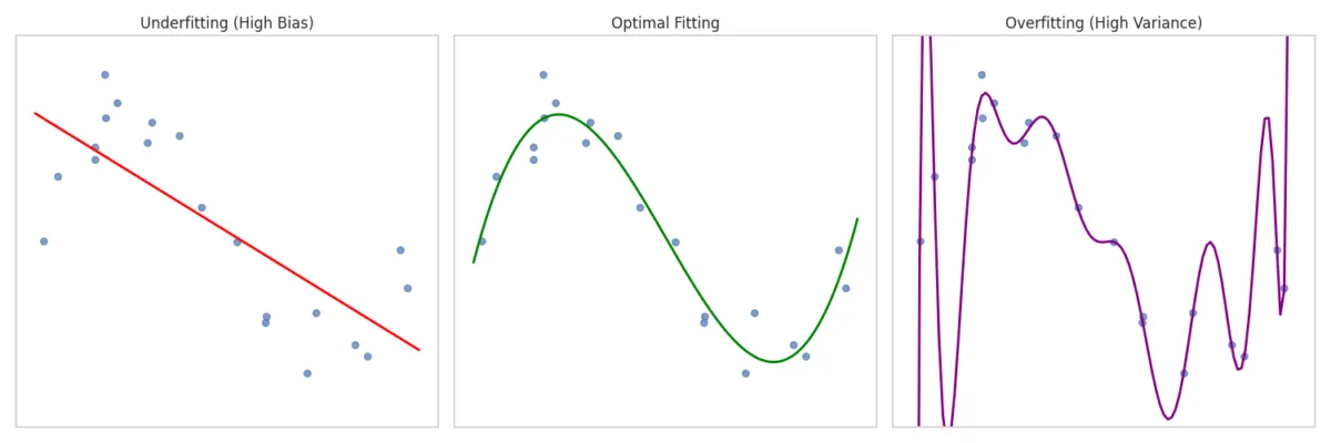
Underfitting & Overfitting
#Regularization
When the model is too complex, i.e. it is overfitting, the variance can be reduced by constraining the model weights. This is called regularization. It works by adding a penalty term to the Loss Function (Residual Sum of Squares [RSS]).
- is the tuning parameter.
- As , coefficients shrink toward zero, reducing variance but increasing bias.
#Ridge Regression ( Regularization)
Ridge adds the squared magnitude of coefficients as the penalty.
Expanding it :
- Shrinks coefficients toward zero but never exactly to zero. It includes all features in the final model (no variable selection).
L2 Regularization (Ridge)
The constraint region is a circle. The RSS ellipses usually hit the circle at a non-axis point, keeping non-zero.
#Lasso Regression ( Regularization)
Lasso (Least Absolute Shrinkage and Selection Operator) adds the absolute value of coefficients.
Expanding it :
- Can shrink coefficients exactly to zero, effectively performing feature selection. It creates sparse models.
L1 Regularization (Lasso)
The constraint region is a diamond. The RSS ellipses often hit the "corners" of the diamond (the axes), forcing some coefficients to zero.
- It is not differentiable at 0.
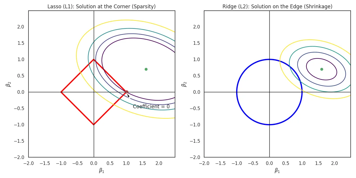
L1 vs L2 regularization
#Elastic Net
Elastic Net combines both and penalties to get the best of both worlds - feature selection (Lasso) and handling correlated features (Ridge).
- Use Case: Ideal when we have high-dimensional data or highly correlated groups of features.
With this, the post on confusion matrix, metrics to evaluate the performance of the model, Bias-Variance Tradeoff and Regularization is completed.