2. ML: Linear Regression
#Regression Problem
It is a statistical process for estimating the relationships between a dependent variable (outcome) and one or more independent variables (features).
- Input : Attribute variables or features (typically numerical values).
- Output : Response variable that is aimed to be predicted.
Objective
The goal is to estimate a function such that .
It is called linear regression because this relation is assumed to be linear with an additive error term representing statistical noise.
#Simple Linear Regression Formulation
For a single feature vector , the regression models is defined as :
- : observed response for -th training example
- : input feature for the -th training example
- : intercept (bias)
- : slope (weight)
- : residual error
This represent the actual training dataset values.
The fitted values or the prediction is :
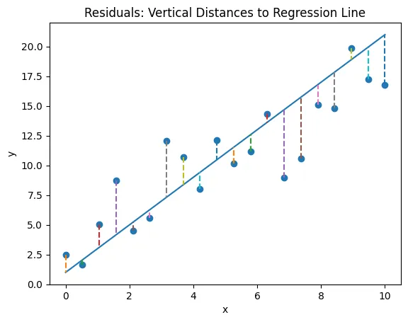
Residuals in linear regression
#Ordinary Least Square (OLS)
It is the method to estimate the unknown parameters () by minimizing the sum of the squares of the differences between the observed dependent variables and the predicted ones by the liner function. Squared error penalizes large errors more than smaller ones.
#Derivation of Sum of Squared Errors (SSE)
Residual Sum of Squares (SSE) cost function is defined as :
Goal
Minimize
To find the optimal and , we take partial derivative w.r.t each parameter and set them to 0.
#1. Derivative w.r.t :
To minimize, the derivative must be equal to 0 :
Since and are constants :
Dividing by :
#2. Derivative w.r.t :
Substitue with :
Rearranging :
Identity : and same is true for .
Thus, numerator becomes :
And thus denominator becomes :
And finally the slope becomes :
And in terms of covariance and variance :
#Sum of Squares Decomposition and
To evaluate the goodness of fit, we decompose the total variability of the response variable.
- SST (Total Sum of Squares) : Measures total variance in observed :
- real vs mean
- SSR (Sum of Squares Regression) : Measures variance explained by the model :
- predicted vs mean
- SSE (Sum of Squares Error) : Measures unexplained variance (residuals) :
- real vs predicted
These are related as :
#Coefficient of Determination ()
represents the proportion of the variance for the dependent variable that's explained by an independent variable.
Also,
- The best model will have .
#Correlation Coefficient ()
For simple linear regression, is the square of Pearson Correlation Coefficient () :
#Types of Errors
Different metrics are used for different purposes :
#1. Mean Squared Error (MSE) :
- Differentiable and useful for optimization.
- Heavily penalizes large outliers (squaring term).
#2. Root Mean Squared Error (RMSE) :
- Same unit as the target variable , making it interpretable.
#3. Mean Absolute Error (MAE) :
- More robust to outliers than MSE, but not differentiable at 0.
#Multiple Linear Regression
When multiple features are present like , the model becomes :
#Vector-Matrix representation
Add a bias term as for the intercept into the weight vector :
- Input Matrix : Dimensions
: -th training example's -th feature.
Weight Vector : Dimensions
- Target Vector : Dimensions
The prediction can be written using the inner product for a single example or matrix multiplication for the whole dataset:
#Closed Form / Normal Form Equation
goal
To find the coefficient , minimize the sum of squared error (SSE).
#Define the cost function
Cost function (quantifies the error between a model's predicted outputs and the actual target values) :
- : optimal value of the parameter.
SSE = which is equal to magnitude of the vector . Due to the fact that :
And since
Thus,
Solving this gives :
The term will give a scalar value of dimension (). And because transpose of a scalar is equal, . Thus,
#Computing the gradient
To find the optimal that minimizes error, we calculate the gradient of with respect to and set it to zero.
- Constant with respect to
- is our variable vector .
- is a constant vector because it doesn't contain .
- The term can be rewritten as the dot product .
- Rule: The derivative of a dot product with respect to one of the vectors is just the other vector.
- is a vector.
- is a square matrix.
- The expression is called a Quadratic Form.
- Rule: The derivative of a quadratic form depends on whether matrix is symmetric.
Another rule followed :
Thus, the final gradient becomes :
#Solving for
Equating the gradient to 0 :
Thus, the closed form or the normal form equation is :
#Limitations
- It requires to be invertible, i.e., the features must not be perfectly correlated.
- For larger data, computation required to compute the inverse will be too large.
#Gradient Descent
When the normal equation becomes too computationally expensive, we use Gradient Descent : an iterative optimization algorithm.
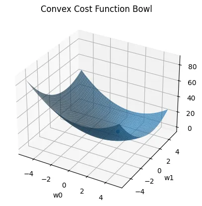
Convex Bowl
#Cost Funtion (Mean Squared Error Form)
- The factor makes the derivative cleaner.
#Update Rule
Update the weights by moving in the opposite direction of the gradient / negative gradient.
- is the learning rate
The gradient for a specific weight is :
#Types of Gradient Descent
| Type | Description | Pros | Cons |
|---|---|---|---|
| Batch GD | Uses all N training examples for every update. | Stable convergence. | Slow for large datasets; memory intensive |
| Stochastic GD (SGD) | Uses 1 random training example per update. | Faster iterations; escapes local minima | High variance updates; noisy convergence |
| Mini-Batch GD | Uses a small batch (b) of examples per update. | Balances stability and speed. | Hyperparameter b to tune |
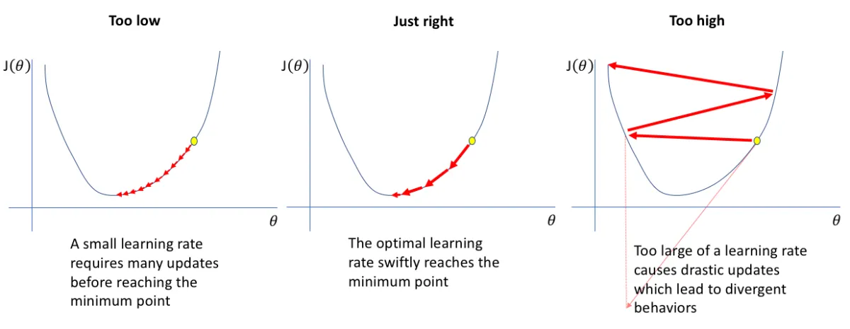
#Learning Rate ()

Different Alpha values result
It is a critical hyperparameter that controls the step size taken towards a minimum of a loss function during optimization
- too small: Convergence is guaranteed but very slow; requires many updates.
- too large: The steps may overshoot the minimum, causing the algorithm to oscillate or diverge (cost increases).
- Optimal : Smoothly reaches the minima.
Learning rate in bowl
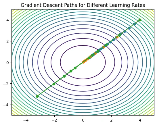
Learning Rate Trajectories
#Worked out examples of Gradient Descent
Problem : Fit : .
Dataset :
- Point 1:
- Point 2:
Initialization :
- Learning Rate .
#Batch Gradient Descent
It calculates gradient using sum over all points ().
- Error :
- Error :
Gradients :
- Because for . Thus, :
Update :
Thus, the model after 1 epoch (1 complete pass through the dataset) is
#Stochastic Gradient Descent (SGD)
It updates after each example.
Iteration 1 :
Pred :
Gradient for as .
- Gradient for as .
- Update :
Thus, the current model is :
Iteration 2
Use the updated weights from Iteration 1.
- Prediction :
- Compute gradients
- Update Weights :
Thus, the final model after 1 epoch is :
With this post on Linear Regression, normal form equation, gradient descent, types of errors, OLS is over.