3. ML: Logistic Regression
#Classification Problem
In supervised learning, when the target variable is discrete or categorical, the task is called Classification. It asks which category? unlike regression which asks how much?.
Given a dataset , where are the features, we seek a function .
In Binary Classification, where :
- : Negative class (e.g., Benign tumor, Non-spam).
- : Positive class (e.g., Malignant tumor, Spam).
#Logistic Regression is a Generalized Linear Model (GLM)
Logistic Regression is a regression model for probabilities. It predicts a continues probability value , which is descretized using a threshold (0.5) to perform classification.
Thus, it is a regression model adapted for classification tasks.
#Deriving Logistic Regression from Linear Regression
Linear model can be adapted for binary classification by mapping the output of the linear equation to the interval . This can be achieved by using the Odds Ratio and the Logit function.
#1. Odds Ratio
The odds of an event occuring is the ratio of the probability of success to the probability of failure .
- The range of the odds is .
#2. Logit (Log-Odds)
The output range of linear regression model is . To map the range of the Odds () to this, take the natural log of the Odds :
This linear relation implies that the log-odds are linear w.r.t the input features .
#3. Sigmoid Function
Isolate in the above equation as it is what we need to find out. For this, the logit function is inverted by raising both side to power of :
Let . Then dividing the numerator and denominator by :
is called the Sigmoid Function.
![Sigmoid Mapping inputs to [0,1]](/static/images/Ml-9.webp)
Sigmoid Mapping inputs to [0,1]
#Extending Binary Models to Multi-Class
As the name suggests, binary model is good for only 2 class problems. For more more than 2 classes a different approach is required.
#One vs All Approach
For classes, we train separate binary logistic regression classifiers. For each class , a model is trained to predict the probability that a data point belongs to that class versus all other classes.
- Treat class as the "Positive" () class.
- Treat all other classes () as the "Negative" () class.
For prediction, we run all classifiers and choose the class that maximizes the probability.
#Softmax Regression / Multinomial Logistic Regression
It models the joint probability of all classes simultaneously. Instead of a single weight vector , we now have a weight matrix of shape (where is the number of features). Each class has its own distinct weight vector .
For a given input we compute a score or logit for each class
Or in vector notation :
#Softmax Function
The sigmoid function maps a single value to . The Softmax function generalizes this by mapping a vector of arbitrary real values (logits) to a probability distribution of values.The probability that input belongs to class is given by:
- It is like a max function but differentiable, hence soft.
- Sum of probabilities is 1.
- Each output value is in interval .
#Loss Function : Maximum Likelihood Estimation (MLE)
#Why not use MSE?
MSE is used in Linear Regression because it creates a bowl-shaped convex curve. No matter where we start on the curve, via Gradient Descent we will eventually reach the absolute bottom (Global Minimum).
However, applying MSE in Logistic Regression which uses a sigmoid function (non-linear function) will result in a non-convex, wavy and complex graph.
Convex Functions
If a line segment between any 2 points of the function does not lie below the graph.
The non-convex curve has many valleys (local minima). If the algorithm starts in the wrong spot, it might get stuck in a shallow valley and think it has found the best solution when it hasn't. Hence, MSE is not used for Logistic Regression.
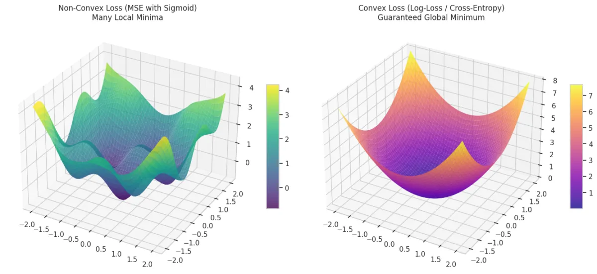
MSE vs Log-Loss
#Binary Cross-Entropy (BCE) Loss
Due to failure of MSE, BCE is derived using Maximum Likelihood Estimation (MLE).
Instead of measuring the distance between the prediction and the target (like MSE), MLE asks a statistical question: What parameters () would maximize the probability of observing the data we actually have?
Assumption : The target follows a Bernoulli Distribution, because the output can only be or .
- If the actual class is 1, we want the model to predict a high probability ().
- If the actual class is 0, we want the model to predict a low probability (which means is high).
This can be compacted to :
Assuming independent training examples, the Likelihood of the parameter is the product of the probabilities of the observed data :
To simplify differentiation and avoid numerical overflow, we maximize the Log-Likelihood . This makes the Product to Summation .
Taking natural log :
But optimization algos are designed to minimize the error, not maximizze the likelihood. Thus, this equation is inverted by adding a negative sign.
Thus, the final Binary Cross-Entropy Loss or the Negative Log-Loss function is :
Thus, the average BCE loss is :
- This is a convex function and thus gradient descent will converge to the global minima.
#Gradient Descent Derivation
Goal
Minimize . For this, the gradient is needed.
#1. Derivative of Sigmoid Function
#2. Derivative of the loss (Chain Rule)
Using only a single example :
Using the chain rule :
- Partial of Loss w.r.t Prediction :
- Partial of Prediction w.r.t Logit :
- Partial of Logit w.r.t Weight :
#3. Combining Terms
The term cancels out, leaving :
#Batch Gradient Descent
Update weights using the average gradient over the entire dataset :
#Stochastic Gradient Descent
Update the weights for each training example individually:
note
This rule is identical in form to the Linear Regression update rule but the definition of has changed from linear () to sigmoid ().
#Binary Logistic Regression is a linear classifier.
To prove that a classifier is linear, we must show that the decision boundary separating the classes is a linear function of the input features (i.e., a line, plane, or hyperplane).
In logistic regression, the probability prediction is given by the sigmoid function applied to a linear combination of inputs.
(logits) is a linear function of the weights and features :
An instance is classified into the positive class () if the predicted probability is greater than or equal to a threshold, typically .
Taking the natural log () of both sides
The decision boundary is the exact point where the classifier is uncertain (probability ), which corresponds to the equation:
- This represents a hyperplane (line in 2D, plane in 3D).
Since the boundary that separates the two classes in the feature space is linear, Logistic Regression is, by definition, a linear classifier.
- While the decision boundary is linear, the relationship between the input features and the predicted probability is non-linear (S-shaped or sigmoidal).
- The "linear" label strictly refers to the shape of the separation boundary in space, not the probability curve.
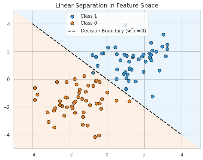
Linear Separation in Feature Space
With this, the post on binary classifiers, logistic regression, Binary Cross Entropy Loss / negative log-loss comes to an end.