11. NLP: Tokenizers
#Tokens & Tokenization
Tokens are the basic unit of data that an LLM processes.
- It can be a whole word, part of a word or even a single char.
- eg. :
token,token+ization," ".
Tokenization is the process of breaking raw texts into individual tokens.
- Since computers can't understand words, tokenization also maps the text to a list of numbers (IDs).
Now lets see different types of tokenizations :
#Word-Level Tokenization
- It seems an intutive approach as words in texts are delimited by spaces so whitespaces makes a natural boundary for tokenization.
- Words are excellent in carrying the sematic meaning.
- eg.
applecarries a specific, dense meaning which is easily understood by both humans and models.
- eg.
- It used primarly in early NLP systems.
But using word-level tokenizations have disadvantages too :
Curse of Dimensionality : Vocabulary size required to cover a large language is immense. There can be tens or hundreds of thousands of unique words in a language or a large, diverse document.
OOV Problem : Out-Of-Vocabulary (OOV) words are those words / tokens which do not appear in training and thus are mapped to a generic token
[UNK]. This results in total loss of information for that term. Thus, it reduces the ability & quality of a model.
To address this vocabulary explosion, other tokenization schemes were explored.
#Character-Level Tokenization
Treat each char as a token.
This results in vocabulary size to collapse to a manageable range ( 256 chars for ASCII or a few thousands for Unicode).
This also addresses the OOV problem as any text can be represented as a sequence of characters who are already classified as tokens.
But it introduces new problems :
Computation Cost : A sentence of just 10 words may have 50 chars. Since the complexity of Self-Attention mechanism is , char-level tokanization increases the training cost drastically.
Lack of Semantics : Individual chars / tokens have little to no semantic meaning (eg.
t,h). Thus, model will have to use significant capacity to compose these chars into meaningful morphological units.
#Subword Tokeniation
- It is a hybird approach that optimally balances efficiecy of word-level models with generalization of char-level models.
Frequency-based decomposition : frequently occuring words are given unique tokens (eg.
the,algorithm) and rare words are decomposed into meaningful sub-units (eg. "tokenization" ->token+##iza+##tion).
- This allows for a vocabulary of manageable size, semantic coverage & morphological generalization.
#Unicode Encoding & Text Representation
In Unicode encoding, every character in every writing system is assigned a unique number.
These numbers are written as :
U+<hexa-decimal no.>.- eg.
U+0061=a.
- eg.
UTF-8is the dominating encoding format currently.- It has a varible-width where chars can occupy between 1 & 4 bytes.
- eg. ASCII chars take 1 byte :
U+0000toU+007F. - eg. Emojis take 4 bytes.
- eg. The emoji : "😊" =
U+1F60A- A byte-level tokeizer will see this as a stream of byte sequences :
[0xF0, 0x9F, 0x98, 0x8A]
- A byte-level tokeizer will see this as a stream of byte sequences :
#Normalization Forms
Canonical Equivalence is the phenomenon where visually identical text can have different binary representations.
Example :
ñcan be represented in 2 ways :- Precomposed : A single code point =
U+00F1 - Decomposed : A sequence of 2 code points :
U+006E(small 'n') +U+0303(combining tilde).
- Precomposed : A single code point =
If the tokenizer treats these differently, then it will learn different / separate embedding for
ñ, fracturing the semantic space.
Thus, Unicode Normalization is employed in tokenization pipeline.
#1. NFD (Normalization Form Decomposition)
Breaks down all composite chars into their base components. Thus, ñ becomes n + ~. It is useful for striping accents.
#2. NFC (Normalization Form Composition)
First decompose the chars and then recompose them into their canonical forms where ever possible. It is generally prefered for final input to the tokenizer to ensure the shortest possible representation of common chars.
#3. NFKC (Normalization Form Compatability Composition)
It handles compatibility chars.
- eg.
ffi=U+FB03is compatible to sequenceffibut not canonically equivalent to it. - Thus, NFKC forces this conversion:
ffi"f", "f", "i".
#Architecture of Tokenization Pipeline
Here we will be discussing about the Hugging Face's tokenizers library.
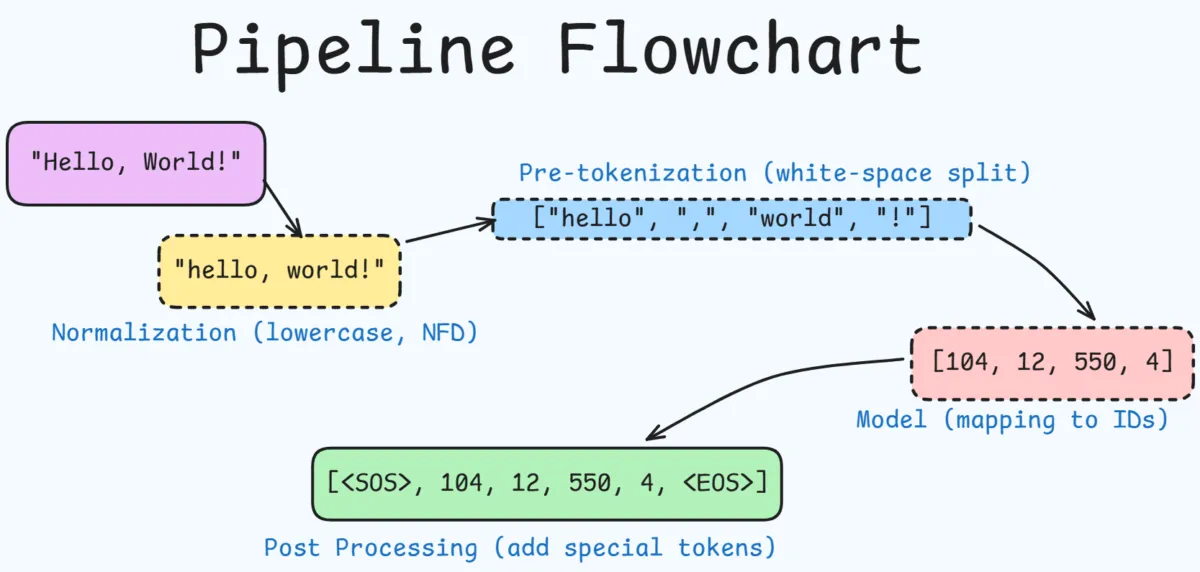
Tokenization is not a monolithic function but modular pipeline consisting of 4 distinct stages :
- Normalization
- Pre-tokenization
- Model
- Post-tokenization
#1. Normalization
Transforms raw input string into clean standard form.
Operations performed :
- Unicode Normalization : Apply NFD, NFC or NFKC.
- Case Folding : Some models use case-insesitive text, so converts the text to lower-case.
- It reduces the vocab size significantly but loses distinction between proper nouns (eg. Apple the company) & common nouns (eg. apple the fruit).
- Strip Accents : Often used in english-centric models.
- Control Character Removal : Strips non-printable chars that might interfere with processing.
#2. Pre-tokenization
This defines an upper bound of a token. It prevents the model from merging parts of 2 distinct words.
- eg. Prevents merging of words :
puctuation&wordif they are adjacent.
It splits the normalized strings into smaller units like words or sub-sentence segements.
Strategies employed are :
Whitespace : Splits on space chars. Used by basic BPE implementations.
Whitespaces + Punctuation : eg.
Hello, world!=["Hello", ",", "world", "!"]. Used by BERT.Byte-Level (GPT-2/GPT-3) : Splits the text based on category.
- Use regular expression to split text into chunks that are alphanumeric strings, strictly numeric or punctuation.
- This prevents merging across categories like a letter and a number.
Metaspace (SentencePiece) : Replaces spaces with a visible char like
_and treats the string as a continuous stream. This delays the splitting decision to the subword model which allows more flexible segmentation.
#3. Model
The core component that performs the actual subword segmentation.
Maps the pre-tokenized words and maps them to a sequence of integers (Token IDs).
- It discovers the optimal subwords units and apply them to the input.
- This is done by specific algos like BPE, WordPiece & Unigram.
- The model must be trained on a corpus to learn the vocabulary and merge rules.
#4. Post-Processing
Adds special tokens required by the model structure like <SOS> (Start of Sequence) & <EOS> (End of Sequence) or <|endoftext|> depending on the model being used.
Other operations :
- Truncation : Cuts the sequence to the max. content length
- Padding : Adds
PADtokens to ensure all sequences in a batch have same length. - Attention Mask : Generates binary masks that tell the model which tokens are real data and which are padding.
Tokenization Pipeline
#Byte Pair Encoding (BPE)
It is the most influential algorithm in the current generation of LLMs.
Core intution : Iterative, frequency-based merging.
It begins with a vocabulary of elementary units (chars) and iteratively merges the most frequently adjacent pair of units into a new, single unit. This process continues until a new pre-defined vocabulary size is reached.
#Training Algorithm
Preparation :
- Corpus is pre-tokenization into words.
- Special end-of-word symbol (eg.
/w) is appended to mark each word's boundaries.
Base Vocabulary :
- Initialize base vocab with all unique chars in corpus.
Counting Pairs :
- Count frequency of every adjacent pair of symbols across all words in corpus.
Merging :
- Identify the pair with highest freq.
- Let the pair be
(A, B). Thus, create a new tokenAB.
Update :
- Add
ABto vocab. - Replace all occurences of
(A, B)in the corpus withAB.
- Add
Iteration :
- Repeat steps 3-5 until the vocab reaches pre-defined (hyperparameter) target size.
#Example :
- Corpus :
["hug", "pug", "pun", "bun", "hugs"] - Base Vocab :
['b', 'g', 'h', 'n', 'p', 's', 'u'] - Pairs :
('u', 'g')appears most frequently. - Thus, new corpus state :
["h", "ug"], ["p", "ug"], ["p", "u", "n"],... - Next frequent pair :
("h", "ug"), ... and so on.
#Inference
The model applies the learned merge rules in the the exact order they were discovered during training.
- It is a greedy, deterministic process.
- Tokenizer scans the words & applies the highest priority merge available repeatedly until no more merges apply.
#Byte-Level BPE
Standard BPE required a base vocab of unicode chars, which has more than 140,000 chars. This makes the vocab prohibitively large which may lead the model to prune rare tokens leading to [UNK] for emojis or foreign scripts.
BBPE solves this by operating on bytes (UTF-8) rather than chars.
- Base vocab is strictly of size 256 (byte values 0-255).
- Since any text can be represented as a sequence of UTF-8 bytes, BBPE can tokeinze any string without introducing
[UNK]tokens.- Thus an emoji or a chinese char can be broken down into its constituent 3 or 4 bytes.
#WordPiece: Likelihood Maxizer
This is the tokenization algo behind BERT and its derivatives. It differes from BPE in its selection criteria.
- BPE : Merges 2 tokens because they appear together frequently.
- WordPiece : Meges tokens only if they are stronglt coupled, i.e., they appear together more often than one would expect by random choice.
#WordPiece Score
WordPiece chooses the merge that maximizes the likelihood of the training data.
For a pair of tokens (u, v), score is :
The actual formula is the frequency one, but it is easier to understand the concept using probability one.
Numerator :
- This is the reality or the observed probability.
- It measures how often do these 2 units appeat together in the text.
Denominator :
- This is the expectation or the Expected Probability under Independence
If 2 events are independent, i.e., they have no relationship, then the probability of them happening together is just the product of their individual probabilities.
- This tells how often token u & v will land next to each other if they were thrown into a bag and pulled out, purely by chance.
#Analysis :
: Pair appear as often as a random chance.
- Thus, no relationship. Don't merge.
: Pair appear less often than random chance.
- They repel each other. Don't merge.
: Pair appear much more often than random chance.
- Strong relationship. Merge.
eg. in a trainig dataset of 1000 total token pairs.
#Case-1 : Popular pair
isappears 100 times. (P = 0.1)itappears 100 times. (P = 0.1)together
isitappears 20 times (P=0.02)BPE sees 20 occurrences, which might be high and it may consisdier merging them.
However, WordPiece score :
- They appear only twice as often as random chance. This is a weak connection.
#Case-2 : Rare pair
zappears 10 times. (P = 0.01)jappears 10 times. (P = 0.01)together
zjappears 9 times. (P = 0.009)BPE sees only 9 occurrences. This is lower than
isit(20 times). Thus, BPE igonres this pair.WordPiece
So, even though they are rare, they are inseparable.
Thus, WordPiece will merge zj before it merges isit.
- It distinguishes between a token at the start of a word and a token inside a word by prefixing tokens inside a word with
##. - eg.
tokenization["token", "##iza", "##tion"]
This allows a model to distinguish between ##able (suffix) & able (word).
#Unigram Language Model: Probabilistic Approach
Unigram algo, introduced in 2018, is used typically within the SentencePiece library.
BPE & WordPiece are bottom-up algorithms, i.e, they start with chars and merge them, Unigram is top-down.
#Probabilistic Model
- The model is based on the fact that a sequence of text is generated by a sequence of subwords .
- Each subword occurs independently.
Thus, the probability of the sequence is the product of probabilities of the constituent subwords :
is the probability of subword in the current vocab distribution.
is the likelihood of the entire corpus
- Likelihood means the probability that the model, with its current vocabulary and token probabilities, would generate the entire training corpus exactly as observed.
The model assumes that text is generated by reapeatedly picking one token at a time from a vocab, each with its own fixed prob.
But it is not known which tokens the corpus should be segmented into nor their probabilities.
#Training via Expectation Maximization (EM)
Goal : To find a vocabulary and the probabilities that maximize the likelihood of the training corpus.
#1. Initialization
- Start with a massive vocab like :
- All substrings in the corpus that occur more than times.
- Vocab generated by 30k BPE merges.
#2. E-Step (Expectation)
For every sentence in the corpus, find the most probable segmentation.
There are multiple possible ways to segement a string :
pug -> ["p", "u", "g"], ["pu", "g"], ["p", "ug"]
To find the best possible segmentation that maximizes likelihood efficiently, Viterbi Algorithm is used.
#Viterbi Algo
Given : a string and a vocabulary with token probabilities .
- A segmenatation is a sequence of tokens that concatenate to .
- As discussed above, under Unigram assumption, probability of segmentation = product of token probabilities.
- The segment is not observed, hence it is a latent variable.
Viterbi Algorithm finds the single segmentation with max probability
- The algorithm calculates the probability of each based on current values and selects the highest.
- It uses Dynamic Programming to find the best segmentation in polynomial time.
So, finally the segmentation that has the highest likelihood under the current model is choosen.
#3. M-Step (Maximization)
Try to pick values that make the current segmentations of the corpus as likely as possible.
- Update the probabilty of each token.
- The probability of a token is how often it occurs divided by the total number of tokens in the segmentation.
If a token appears many times in the segmentation, it gets a higher probability, thereby increasing the likelihood of the observed corpus.
#4. Pruning (Feature Selection)
For every token in the vocab, the algo calculates a Loss :
- The loss is the actual log-likelihood values :
This measures how much the total likelihood of the corpus would decrease if token were removed.
- Tokens that effectively capture common patterns will have a high loss.
- Removing them forces the model to use lower-probability sequences.
- Redundant tokens will have low loss.
Thus, algo removes bottom % (eg. 20%) tokens with the lowest loss.
#5. Convergence
Repeat step 2-4 until the vocab size reaches the desired size.
Example
#Vocab is :
papa papa
Made up probabilities :
| Token | P(x) |
|---|---|
| p | 0.15 |
| a | 0.15 |
| pa | 0.10 |
| ap | 0.10 |
| papa | 0.10 |
| pap | 0.10 |
| apa | 0.10 |
| p a p a (char-level) total | (remaining) |
Target size = 4
#1. Initial Vocab :
p, a
pa, ap
papa, pap, apa
etc.
#2. E-Step
p+a+p+a: P = = 0.0005pa + pa: P = = 0.01papa: P =pap + a: P = = 0.015p + apa: P = = 0.015
Hence, best segmentation is : papa with prob. = 0.10
Hence the vocab becomes :
[papa] [papa]
#3. M-Step
New prob :
| Token | New P(x) |
|---|---|
| papa | 2/2 = 1.0 |
| Others | 0 |
#4. Prunning
- Removing
papawill lead to huge likelihood crash. Thus, keep it. - Removing other has no effects.
So, new vocab is :
papa, pa, p, a
Stop, since target size is achieved, otherwise would have kept on going on.
This concludes this post on tokenizers, with main conclusions being :
- Byte-level BPE is the standard for generative models due to its simplicity and OOV robustness.
- Unigram offers better compression and token efficiency.
- Pipeline is an important part as BPE model with poor normalization or pre-tokenization will perform poorly.