3. Neural Nets: Activation Functions
Activation Functions
- It is used to introduce non-linearity into the neural network.
- This allows to model complex relatioships in data.
Why activation functions are needed ?
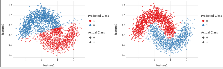
- The data on left can be modelled by using a linear function.
- The data is linearly separable.
- linear activation / no activation is sufficient.
- But the data on right can’t be modelled using linear function
- Linear model will fail here because it can only create a straight-line decision boundary.
- Therefore, a non-linearity is required to model the data.
- Without activation functions, deep networks behave like a simple linear model, limiting their capability.
Types of Activation functions
import torch
import torch.nn as nn
1. Linear Activation Funtion
\[f(x) = ax + b\]- Output is proportional to input
- Doesn’t introduce non-linearity.
- Rarely used.
PyTorch Implementation :
linear_activation = nn.Identity()
x = torch.tensor([1.0, 2.0, 3.0])
output = linear_activation(x)
2. Sigmoid Activation (σ)
\[f(x) = \frac{1}{1 + e^{-x}}\]- Output in range (0,1).
- Used in binary classification problems.
-
Can be interpreted as probabilities (used in logistic regression).
- Drawback
- Vanishing gradient problem
- When inputs are large/small, gradients become very small.
- Vanishing gradient problem
PyTorch Implementation :
sigmoid = nn.Sigmoid()
x = torch.tensor([-1.0, 0.0, 1.0])
output = sigmoid(x)
3. Hyperbolic Tangent (Tanh)
\[f(x) = \frac{e^{x} - e^{-x}}{e^{x} + e^{-x}}\]- output in range in (-1,1)
- Centered around 0, helps in faster convergence
-
Usefull for hidden layers in deep networks.
- Drawback
- Vanishing Gradient Problem (better than sigmoid)
- Computationally expensive
PyTorch Implementation :
tanh = nn.Tanh()
output = tanh(x)
4. Rectifed Linear Unit (ReLU)
\[f(x) = max(0,x)\]- most widely used activation function.
- output in range [0,∞).
- Solves vanishing gradient problem (because no exponentials).
- efficient computation.
-
Sparse activation (many neuron output 0).
- Drawback
- Dying ReLU Problem (Neurons that output zero remain inactive).
- Not centered around zero.
PyTorch Implementation :
relu = nn.ReLU(x)
output = relu(x)
5. Leaky ReLU
\[f(x) = \begin{cases} x, & \text{if } x \geq 0 \\ \alpha x, & \text{if } x < 0 \end{cases}\]- output in range (-∞,∞).
- modified ReLU, allows a small gradient for negative inputs
- default α = 0.01
-
prevents Dying ReLU Problem
- Drawback
- Requires tuning of slope
PyTorch Implementation :
leakyrelu = nn.LeakyReLU(negative_slop=0.01)
ouyput = leakyrelu(x)
6. Parametric ReLU (PReLU)
\[f(x) = \begin{cases} x, & \text{if } x \geq 0 \\ \alpha x, & \text{if } x < 0 \end{cases}\]- output in range (-∞,∞).
- Unlike Leaky ReLU, α is learned during training.
- Same equation as Leaky ReLU
- Adaptive slope improves performance
-
Avoids dying ReLU issue.
- Drawback
- Extra parameter α increases computation.
PyTorch Implementation :
prelu = nn.PReLU()
output = prelu(x)
7. Exponential Linear Unit (ELU)
\[f(x) = \begin{cases} x, & \text{if } x \geq 0 \\ \alpha (e^x - 1), & \text{if } x < 0 \end{cases}\]- output in range (-∞,∞).
- smooths out the output for negative values
- Avoids dying ReLU.
-
Helps with vanishing gradients
- Drawback
- More computationally expensive.
PyTorch Implementation :
elu = nn.ELU(alpha=1.0)
output = elu(x)
8. Softmax
\[\sigma (x_i) = \frac{e^{x_i}}{\sum_{j} e^{x_j}}\]- output in range (0,1).
- Used in the final layer of classification networks. (Multi- CLass)
- Outputs probabilities.
-
Converts logits(unnormalized scores) into probabilities summing to 1.
- Drawback
- Can be overconfident in predictions (sensitive to large values)
PyTorch Implementation :
softmax = nn.Softmax(dim=1) # axis 1 across row
output = softmax(torch.tensor([[1.0, 2.0, 3.0]]))
Summary
- Activation functions introduce non-linearity to neural networks.
- ReLU is widely used in deep learning due to its efficiency.
- Tanh is preferred over Sigmoid due to its zero-centered outputs.
- Softmax is essential for multi-class classification tasks.
Choosing the right activation function is crucial for model performance and convergence stability.
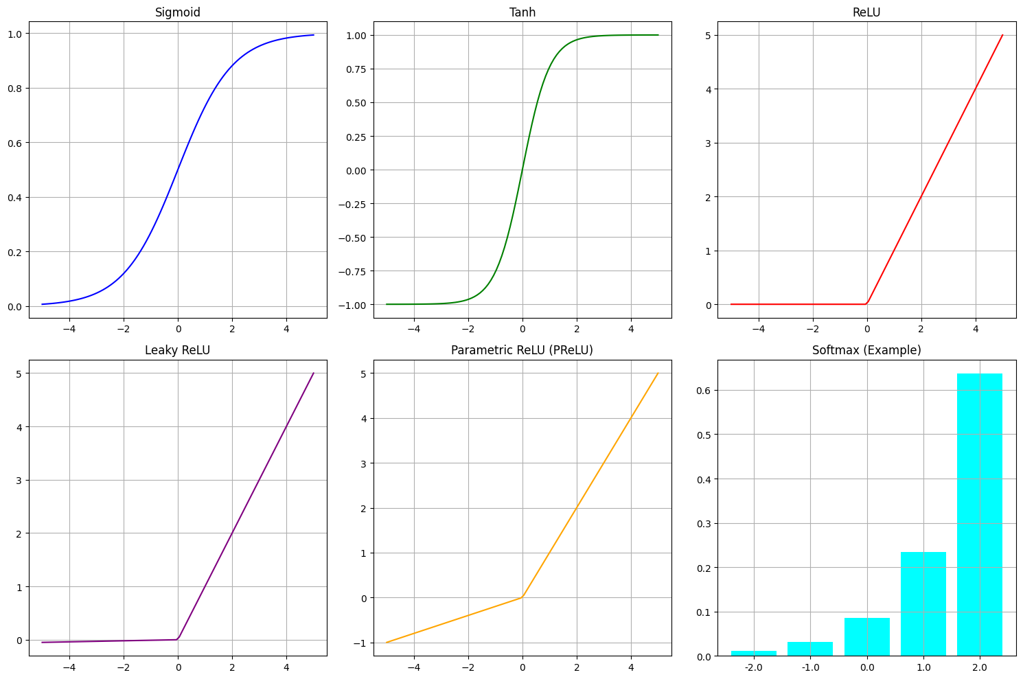
Plot of some of the activation functions