4. Neural Nets: Loss and Optmization
import torch.nn as nn
Loss Functions
- measure how well a model’s predictions align with the actual outputs.
-
the choice of loss function depends on the task :
-
Loss Functions for Regression
-
Mean Squared Error (MSE)
- \[MSE = \frac{1}{n} \sum_{i=1}^{n} (y_i - \hat{y}_i)^2\]
- mean of squares of differences of predicted and actual values
- Penalizes large errors more than small errors.
-
Sensitive to outliers.
- Pytorch Implementation
loss_fn = nn.MSELoss()L2 Lossis the same as MSE but without the mean part
-
Mean Absolute Error (MAE)
- \[MAE = \frac{1}{n} \sum_{i=1}^{n} | y_i - \hat{y}_i |\]
-
more robust to outliers
- Pytorch Implementation
loss_fn = nn.L1Loss()
-
-
Loss Functions for Classification
-
Cross-Entropy Loss (Softmax + Log Loss)
- \[L = - \sum_{i=1}^{n} y_i log(\hat{y}_i)\]
-
for multiclass classification
- Pytorch Implementation
loss_fn = nn.CrossEntropyLoss() -
Binary Cross-Entropy Loss (Sigmoid + Log Loss)
- \[BCE = - \frac{1}{n} \sum_{i=1}^{n} [ y_i log(\hat{y}_i) + (1 - y_i) log(1-\hat{y}_i) ]\]
-
for binary classification
- Pytorch Implementation
loss_fn = nn.BCELoss()
-
-
Optimizers
- Optimizers adjust model parameters (weights and biases) to
minimize the loss functionby computing gradients and updating weights accordingly.
Strategies to optimize the loss function
1. Random Search
- Try out different random values for parameters.
- The set of parameters which give the least loss will be the optimum parameters
- Accuracy : 15.5% (1000 tries)
2. Numeric Gradient / Finite Difference Approximation
- Gradient
- It is the collection of partial derivatives / slopes, organized into a vector, that tells you how a multi-variable function changes.
- \[\frac{df(x)}{dx} = \lim_{h\to 0} \frac{f(x+h) - f(x)}{h}\]
- Numerical gradient computation is based on finite difference approximation.
- It estimates the gradient (derivative) of a function f(x) by slightly perturbing (modifying) x and measuring the change in f(x).
-
This method does not require explicit differentiation, making it useful for gradient checking.
- Drawbacks :
- slow
- gives approximate answers, thus may have errors
- Requires function evaluation multiple times
3. Analytic Gradient
- Uses calculus to derive exact gradients.
- Loss is a function of
W - \[L_i=\sum_{j\neq y_i} max(0,s_j-{s_y}_i+1)\space and\space s=Wx\]
- Goal is to find those parameter W* which minimies the loss function.
- Minima of function implies the gradient of Loss function w.r.t its weight is minimum.
- Goal is to minimize \(\nabla_W\space L\)
- This method is direct and finds the exact gradient value. No approximation
- Very fast
Gradient Check :
After doing analytic gradient, check the results with your results from numeric gradient.
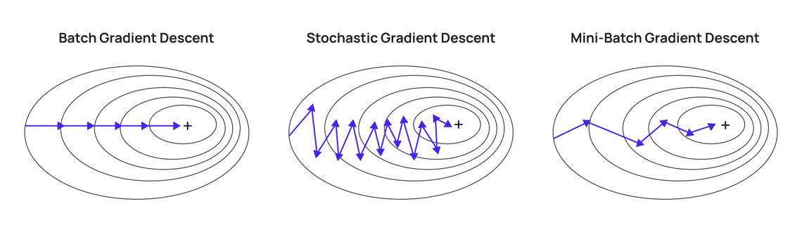
4. Gradient Descent / Vanilla Gradient Descent / Batch Gradient Descent
- Uses the entire batch / dataset to train.
- Process of repeatedly evaluating the gradient and then performng a parameter update
-
\[\theta = \theta - \alpha \nabla J(\theta)\]
- \(\theta\) : model parameters
- \(\alpha\) : learning rate
- \(\nabla J(\theta)\) : gradient of the loss function
- The gradient of a function always points in the direction of the steepest ascent (increase in function value).
- In gradient descent, we move in the opposite direction of the gradient to minimize the function.
Calculations:
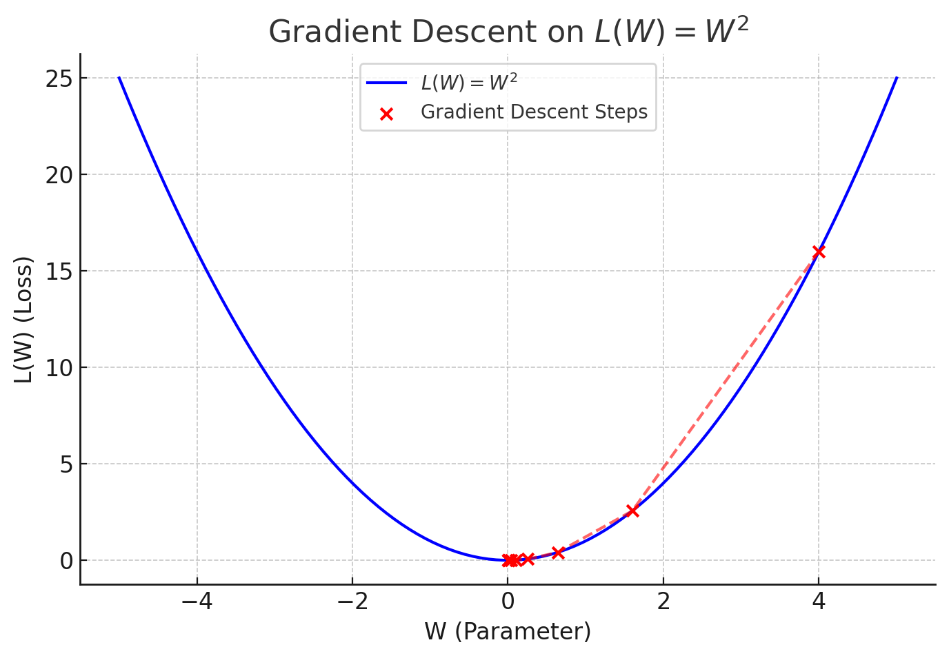
\(L(W) = W^2\)
- The gradient descent update rule is: \(W^{(t+1)} = W^{(t)} - \alpha \nabla_W L(W)\)
- \(\nabla_W L(W) = 2W\) (Gradient of the function)
- \(\alpha = 0.3\) (Learning rate)
Initial value: \(W^{(0)} = 4\)
- Step-by-Step Parameter Updates
Initially
\(W^{(0)} = 4\)
\(\nabla_W L(W^{(0)}) = 2(4) = 8\)
\(W^{(1)} = 4 - 0.3 \times 8 = 4 - 2.4 = 1.6\)Step 1
\(W^{(1)} = 1.6\)
\(\nabla_W L(W^{(1)}) = 2(1.6) = 3.2\)
\(W^{(2)} = 1.6 - 0.3 \times 3.2 = 1.6 - 0.96 = 0.64\)Step 2
\(W^{(2)} = 0.64\)
\(\nabla_W L(W^{(2)}) = 2(0.64) = 1.28\)
\(W^{(3)} = 0.64 - 0.3 \times 1.28 = 0.64 - 0.384 = 0.256\)Step 3
\(W^{(3)} = 0.256\)
\(\nabla_W L(W^{(3)}) = 2(0.256) = 0.512\)
\(W^{(4)} = 0.256 - 0.3 \times 0.512 = 0.256 - 0.1536 = 0.1024\)
Python implementation :
# x = training data
# L() = loss func
# lr = learning rate
for epoch in range(no_steps):
    pred = model(x)
    loss = L(pred, gt)
    W_grad = grad_eval(loss)
    W = W - lr * W_grad
- Learning Rate (\(\alpha\)) :
- it decides how many steps or how far to go
- Large LR :
- faster convergence
- chances to overstep and overshoot the minima
- Small LR :
- slower convergence
- Drawbacks :
- For a large dataset (millions of data), loss function will be computed over the whole dataset, for just one parameter update
- It will become computationally expensive
5. Stochastic Gradient Descent (SGD)
- Training data is divided into sets of batches
- SGD uses only one random data point (or a small batch of data points) at each iteration.
- This makes the computation much faster.
- It is also quite noisy.
Pytorch implementation
model = create_model()
optimizer = torch.optim.SGD(model.parameters(), lr=1e-4)

for input_data, labels in train_dataloader:
    preds = model(input_data)
    loss  = L(preds, labels) #finding out loss
    loss.backward() #perform backprop
    optimizer.step() #updates the weights by taking step
    optimizer.zero_grad() #reset the gradients to avoid adding up
6. Mini-Batch Gradient Descent
- Instead of using a single sample (SGD) or the entire dataset (Batch GD), Mini-Batch GD updates the weights using a small random subset (batch) of the data.
- It updates the models parameter after computing the gradient on a small batch of training data.
PyTorch Implementation
from torch.utils.data import DataLoader, TensorDataset

# Creating Mini-Batches
dataset = TensorDataset(X, y)
batch_size = 2  # Mini-batch size
dataloader = DataLoader(dataset, batch_size=batch_size, shuffle=True)

# Model, Loss, and Optimizer
model = nn.Linear(1, 1)
criterion = nn.MSELoss()
optimizer = optim.SGD(model.parameters(), lr=0.01)

# Training Loop (Mini-Batch GD)
for epoch in range(100):
    for batch_X, batch_y in dataloader:  # Iterating over mini-batches
        optimizer.zero_grad()
        y_pred = model(batch_X)
        loss = criterion(y_pred, batch_y)
        loss.backward()
        optimizer.step()
    if (epoch+1) % 20 == 0:
        print(f'Epoch [{epoch+1}/100], Loss: {loss.item():.4f}')
- It balances speed and stability.
Problems with SGD
- updates the model parameters using gradients computed from a single randomly chosen data point (or a small mini-batch) rather than the full dataset.
- This introduces stochasticity (presence and influence of randomness or unpredictability in a model) in the updates, causing fluctuations in the optimization path.
Thus SGD has high variance.
- when the loss function has different curvatures in different directions i.e., when the function is steep in one direction and shallow in another
- Fast Changes in One Direction (Steep Slope)
- The gradient is large, so the updates are big in this direction.
- The algorithm overshoots and oscillates back and forth.
- Slow Changes in Another Direction (Flat Slope)
- The gradient is small, so updates are tiny in this direction.
- The algorithm progresses very slowly along this axis.
- Since SGD moves in the direction of the gradient, it takes large steps in the steep direction and small steps in the shallow direction.
- Fast Changes in One Direction (Steep Slope)
This causes the optimization path to look like a zig-zag, wasting a lot of time oscillating instead of moving efficiently toward the minimum.
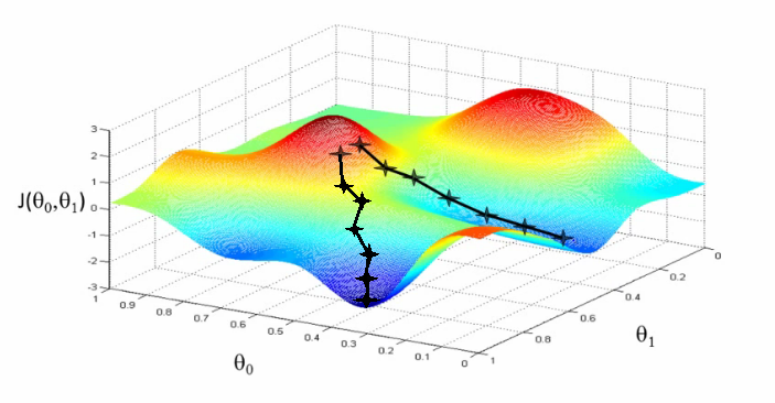
- If the loss function has local minima or saddle point
Since that point has zero gradient, the gradient descent will stop and the optimizer gets stuck, in the case of local minima.
7. SGD with Momentum
Physics Intution behind it
- SGD can be visualized as a person walking down a hill.
- In standard SGD, the person carefully steps in the direction of the steepest descent at each step.
- However, this process can be slow, and the walker might struggle with small dips and oscillations.
- With Momentum is like rolling a heavy ball down the hill.
- Instead of stopping at every step to reassess the direction, the ball carries inertia.
- It allows it to move more smoothly and push through small obstacles, accelerating descent in flatter regions.
Mathematical form
- In vanilla SGD, updates are made solely based on the current gradient.
- But SGD with momentum introduces a velocity component that accumulates past gradients to guide updates more effectively.
- The update equations are:
- \[v_{t+1} = \rho v_t + \nabla f(x_t)\]
- \[x_{t+1} = x_t - \alpha v_{t+1}\]
- \(v_t\) : velocity (actual moving average of past gradients used to update parameters / accumulates past gradients.)
- It acts as a smoother, reducing variance in gradient updates.
- It accelerates descent in directions where gradients are consistently pointing.
- \(\rho\) : momentum (determines how much of the previous velocity is retained)
- It is a scalar.
- typically 0.9
- Higher value implies means stronger past gradient influence.
- Instead of using just the current gradient \(\nabla f(x_t)\) , incorporates \(\rho v_t\) which helps smooth out updates and speed up convergence.
Why Does Momentum Improve SGD?
- Faster Convergence on Long Slopes
- When moving in a consistent direction, momentum accumulates past gradients, effectively accelerating progress.
- Reduction in Oscillations
- In regions with high curvature (e.g., narrow ravines), vanilla SGD tends to oscillate back and forth, slowing convergence.
- Momentum dampens these oscillations by averaging past gradients.
- Ability to Overcome Local Minima and Plateaus
- Unlike standard SGD, which might get stuck in shallow local minima or plateaus, momentum enables the optimizer to “roll through” them due to its accumulated inertia, making it more robust in complex landscapes.
Python Implementation
v_x = 0 #initially no velocity because no gradient is calculated yet
for epoch in range(no_steps):
    for input_data, labels in training_dataloader: # dataloader divides the data into batches
        pred = model(input_data)
        loss = L(pred, labels)
        W_grad = eval_grad(loss)
        v_x = rho * v_x + W_grad
        W -= lr * v_x
PyTorch implementation
optimizer = optim.SGD(model.parameters(), lr=0.01, momentum=0.9)
8. Nesterov Momentum
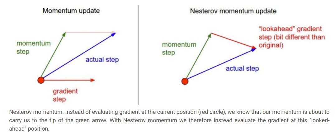
-
Instead of computing the gradient at the current position, Nesterov Momentum “looks ahead” by first making a partial update using the momentum term and then computing the gradient at this “lookahead” position.
- \[v_{t+1}=\rho v_t-\alpha \nabla f(x_t+\rho v_t)\]
- \[x_{t+1}=x_t+v_{t+1}\]
- It prevents overshooting
- Faster convergence
Python Implementation
import numpy as np

# Function to optimize (example: f(x) = x^2)
def gradient(x):
    return 2 * x  # Derivative of x^2

# Initialize parameters
x = 5.0  # Starting point
alpha = 0.1  # Learning rate
rho = 0.9  # Momentum coefficient
v = 0  # Initial velocity

# Perform gradient descent with Nesterov momentum
for i in range(50):
    lookahead_x = x + rho * v  # Lookahead step
    grad = gradient(lookahead_x)  # Compute gradient at lookahead position
    v = rho * v - alpha * grad  # Update velocity
    x = x + v  # Update parameter
9. AdaGrad (Adaptive Gradient Algorithm)
- Instead of using a fixed learning rate 𝛼, Adagrad scales the learning rate based on the sum of past squared gradients.
- Parameters with larger gradients get smaller updates, while parameters with smaller gradients get larger updates.
- \(G_t = \sum_{i=1}^{t} g_i g_i^T\) : accumulated outer product of gradients (a full matrix instead of a scalar sum).
- \(g_t\) : gradient at time t
- \[\theta_{t+1} = \theta_t - \frac {\alpha} {\sqrt G_t} g_t\]
for epoch in range(no_of_epochs):
	for input_data,labels in training_dataloader: #dataloader divides everything into batches
		pred=model(input_data)
		loss=L(pred,truth_values)
		W_grad=evaluate_gradient(loss)
		grad_sq+=W_grad**2
		weights-=learning_rate*W_grad/(np.sqrt(grad_sq)+1e-7)
PyTorch Implementation
optimizer = optim.Adagrad(model.parameters(), lr=0.01)
10. RMSProp (Root Mean Square Propagation)
- It is an adaptive learning rate optimization algorithm.
- It helps mitigate issues related to vanishing and exploding gradients by adjusting the learning rate for each parameter dynamically.
-
Incorporates a moving average of squared gradients to normalize updates.
-
\[E[g^2]_{t+1}=\beta E[g^2]_t+(1-\beta)g(x_t)^2\]
- E[…] : mean or average or Expected value
- g : gradient
- \(\beta\) : decay rate momentum
- typically = 0.9
- determines how much past gradients influence the current update
- RMSprop balances between past and present gradients to smooth learning rate updates.
- Higher β → More weight to past values, smoother updates.
- Lower β → More weight to recent values, more responsive but noisier updates.
Python Implementation
for epoch in range(no_of_epochs):
	for input_data,labels in training_dataloader: #dataloader divides everything into batches
		pred=model(input_data)
		loss=L(pred,truth_values)
		W_grad=evaluate_gradient(loss)
		grad_sq=decay_rate*grad_sq+(1-decay_rate)*(W_grad**2)
		weights-=learning_rate*W_grad/(np.sqrt(grad_sq)+1e-7)
PyTorch Implementation
optimizer = torch.optim.RMSprop(model.parameters(), lr=0.001, alpha=0.9, eps=1e-08)
11. Adam (Adaptive Moment Estimation)
- It is an adaptive learning rate algorithm.
- This means it dynamically adjusts the learning rate for each individual parameter within a model, rather than using a single global learning rate.
-
It combines ideas from both momentum and RMSprop
-
Momentum (First Moment Estimate) (mt)
- Computes an exponentially decaying average of past gradients (similar to momentum).
- Helps in accelerating convergence and overcoming noisy gradients.
- \(m_t = \beta_1 * m_{t-1} + (1-\beta_1) * g_t \rightarrow\) from Momentum
-
Adaptive Learning Rate (Second Moment Estimate) (vt)
-
- Computes an exponentially decaying average of past squared gradients (similar to RMSprop). Helps in scaling learning rates appropriately for each parameter.
- \(v_t = \beta_2 * v_{t-1} + (1-\beta_2) * g_t^2 \rightarrow\) from RMSProp
-
-
Bias Correction
- Since both \(m_{t-1} \quad and \quad v_{t-1}\) are initialized as zero vectors, Adam applies bias correction to compensate for initial estimates.
- \[\hat{m}_{t+1} = \hat{m_t}-\alpha m_t\]
- \[\hat{v}_{t+1}=\hat{v}_t-\frac{\alpha}{\sqrt{\hat{v}_t+\epsilon}}g(v_t)\]
- Update rule for Adam
- \[x_{t+1}= x_t- \frac{(\alpha * \hat{m}_t)}{\sqrt{(\hat{v}_t + \varepsilon)}}\]
-
$m_t$ is the bias corrected first moment estimate and $v_t$ is the bias corrected second estimate.
-
$β^1$ (exponential decay rate for the first moment estimate): 0.9.
- $β^2$ (exponential decay rate for the second moment estimate): 0.999.
Python Implementation
first_moment = 0
second_moment = 0
for t in range(1, num_iterations):
    dx = compute_gradient(x)
    first_moment = beta1 * first_moment + (1 - beta1) * dx
    second_moment = beta2 * second_moment + (1 - beta2) * dx * dx
    first_unbias = first_moment / (1 - beta1 ** t)
    second_unbias = second_moment / (1 - beta2 ** t)
    x -= learning_rate * first_unbias / (np.sqrt(second_unbias) + 1e-7)
PyTorch Implementation
optimizer = optim.Adam(model.parameters(), lr=0.001)
Learning Rate Scheduling
Adjusting learning rate dynamically improves training:
- Step Decay: Reduce learning rate at fixed intervals.
- Exponential Decay: Gradual decrease.
- ReduceLROnPlateau: Adjusts learning rate when validation loss stops improving.
PyTorch Implementation:
scheduler = optim.lr_scheduler.StepLR(optimizer, step_size=10, gamma=0.1)
Summary
| Optimizer | Key Feature |
|---|---|
| SGD | Fast, high variance |
| Momentum | Smooths updates |
| Adagrad | Adaptive learning rate |
| RMSprop | Solves Adagrad’s problem (excessive learning rate decay) |
| Adam | Combines Momentum & RMSprop |
- In practice, Adam is a default choice.
- SGD+Momentum might beat Adam but might require extra fine tuning.