Multi Layer Preceptron (MLP)

Importing Libraries

import torch
import torch.nn as nn
import torch.optim as optim
import torchvision
import torchvision.transforms as transforms
import matplotlib.pyplot as plt

import torch.optim as optim : For optmization.
import torchvision.transforms as tranforms : For preprocessing data (images).

Dataset

MNIST Dataset

60,000 training images and 10,000 test images.
Each image is 28×28 pixels and represents a handwritten digit from 0 to 9.
Images are grayscale, meaning each pixel has a value between 0 and 255.
Task: Build an MLP to classify digits from 0 to 9.
Dataset is available in torchvision.datasets.MNIST.

Preprocessing

Applying transformations to the image.

transform = transforms.Compose([
    transforms.ToTensor(),  # Convert images to PyTorch tensors
    transforms.Normalize((0.5,), (0.5,))  # Normalize to range [-1, 1]
])

transforms.Compose : used to compose several transforms together.
transforms.ToTensor() : Converts the image to a PyTorch tensor and scales pixel values from [0, 255] to [0, 1].
transforms.Normalize((0.5,), (0.5,)) :
- applies : \(x_{normalized} = \frac{x - 0.5}{0.5}\)
- This transforms values from [0,1] → [-1,1].
Thus, the image’s pixel values are now present in tensors, centered around 0.

Loading the data

train_dataset = torchvision.datasets.MNIST(
    root='./data', train=True, transform=transform, download=True
)
test_dataset = torchvision.datasets.MNIST(
    root='./data', train=False, transform=transform, download=True
)

train_loader = torch.utils.data.DataLoader(train_dataset, batch_size=64, shuffle=True)
test_loader = torch.utils.data.DataLoader(test_dataset, batch_size=64, shuffle=False)

train=True # or train=False : determines whether we want training set or test test
transform=transform : applies a set of transformations defined above
download=True : downloads the dataset if it is not found in the root directory.
train_loader = torch.utils.data.DataLoader(train_dataset, batch_size=64, shuffle=True)
- DataLoader : it is a class from torch.utils.data that loads data in mini-batches, shuffles it (if needed), and provides an iterable over the dataset.
- batch_size=64 :
  - Defines the number of samples to be loaded in each batch.
  - Here, 64 means that during training, each iteration will process 64 images at once instead of a single image.
  - Reduces computational overhead by performing matrix operation on a batch instead of single sample.
  - Batch gradient descent.
- shuffle=True : shuffles the dataset at every epoch before creating batches.
  - Prevents the model from learning a fixed order of data, leading to better generalization.
  - Reduces the risk of overfitting on specific patterns in the data order.

Visualizing the data

examples = iter(train_loader) # converts DataLoader into an iterator
images, labels = next(examples) # Get the next batch of images and labels

for i in range(6):
    plt.subplot(2, 3, i+1)  # creates a 2-row, 3-column grid layout for plotting.
    plt.imshow(images[i][0], cmap = 'gray')
    plt.title(f'Label : {labels[i].item()}')  # extracts the numeric label for the image.
    plt.axis('off')     # removes the axis
plt.show()

next(examples) : Each time it is called, it retrieves the next batch from train_loader.
images[i][0] :
- images[i] : selects the i-th image from the batch
- images[i][0] extracts the first (and only) channel, as grayscale images have only one channel (shape: [1, height, width]).

Defining the MLP model

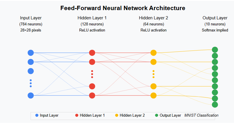
MlP model will consists of the following layers :

Input Layer
- Images in MNIST are of the shape (1, 28, 28)
- 28x28 = 728 neurons
- Flattened images
  
  In PyTorch (channels, height, width) but in TensorFlow/Keras (height, width, channels)
Hidden Layer 1
- 128 neurons
- ReLU activation
Hidden Layer 2
- 64 neurons
- ReLU activation
Output Layer
- 10 neurons
- One neuron for each no [0, 1, …, 9]
- Softmax activation

How to Choose the Number of Neurons?

Start with a simple architecture (like 128 → 64).

Use heuristics:

Keep neurons between input and output sizes.

Decrease neurons layer-by-layer for feature compression.

Experiment:

Too few neurons → underfitting (poor accuracy).

Too many neurons → overfitting (memorizing training data).

Use validation accuracy to tune the model.

class MLP(nn.Module):
    def __init__(self, input_size = 28*28, hidden_size1 = 128, hidden_size2 = 64, output_size = 10): # initializes the network architecture.
        super().__init__()
        self.fc1 = nn.Linear(input_size, hidden_size1) # First hidden layer / Input layer
        self.relu1 = nn.ReLU() # activation func. for first layer
        self.fc2 = nn.Linear(hidden_size1, hidden_size2) # Second hidden layer
        self.relu2 = nn.ReLU() # activation func. for second layer
        self.fc3 = nn.Linear(hidden_size2, output_size) # Output layer

    def forward(self, x):   #  defines how the input data flows through the network.
        x = x.view(x.size(0), -1) # Flatten 28x28 image into 784-dim vector
        x = self.relu1(self.fc1(x))
        x = self.relu2(self.fc2(x))
        x = self.fc3(x)
        return x

x = x.view(x.size(0), -1)
- If x is a batch of images of shape (batch_size, 1, 28, 28),
- .view(x.size(0), -1) reshapes it to (batch_size, 784), ` - Flattening each 28×28 image into a 784-dimensional vector.
- Let x be [64, 1, 28, 28] (batch, channel, height, width)
  - x.size(0) will give the batch size (= 64)
  - Total elements = 64 * 1 * 28 * 28 = 50,176
  - -1 allows to automatically calculate the appropriate size for second dimension based on the tensor’s total elements and other specified dimensions.
  - Second dimension = Total elements ÷ First dimension = 784
- Final tensor shape = [64, 784]
self.fc1 = nn.Linear(input_size, hidden_size1)
- A fully connected layer (FC) that takes an input of size input_size (784) and outputs a vector of size hidden_size1 (128).
- Mathematically, this layer computes:
  - \[h_1 = W_1x + b_1\]
  - where :
    - x is the input vector (size: 784)
    - \(W_1x_1\) is a weight matrix (size: 128 × 784)
    - \(b_1\) is a bias vector (size: 128)

Loss Function

Cross-Entropy Loss

\[Loss = - \sum y_i \log(\hat y_i)\]

criterion = nn.CrossEntropyLoss()

Internally it it computed as :

\[CrossEntropyLoss = − \sum y_{true} ⋅ \log(Softmax(y_{pred}))\]

y_pred are the raw logits from the model.
Softmax converts logits into probabilities.
Negative log-likelihood computes the loss.

If cuda (GPU) is available then switch to cuda or else use CPU

device = torch.device("cuda" if torch.cuda.is_available() else "cpu")
model = MLP().to(device)

Optimizer

Adam

It updates model’s parameters efficiently.

optimizer = optim.Adam(model.parameters(), lr=0.001)

Training the model

Steps involved in training process :

Forward Pass : compute predictions
Calculate Loss : compare prediction with actual labels
Backward Pass : compute gradients using backpropagation
Update Weights : Adjust model parameters

num_epoch = 20

for epoch in range(num_epoch):
    for images, labels in train_loader:
        images, labels = images.to(device), labels.to(device) 

        # Forward pass
        outputs = model(images)
        loss = criterion(outputs, labels)

        # Backward pass
        optimizer.zero_grad()
        loss.backward() # backpropagation
        optimizer.step()

    print(f"Epoch [{epoch+1}/{num_epoch}], Loss: {loss.item():.4f}")

images, labels = images.to(device), labels.to(device)
- Moves images and labels to the specified device (CPU or GPU) for faster computation.
optimizer.zero_grad()
- Clears previous gradients before computing new ones.
- Without this step, gradients would accumulate across batches, leading to incorrect updates.
optimizer.step()
- performs a single optimization step
- Updates the model’s weights using the optimizer
- adjusts the weights in the direction that minimizes the loss.

Evaluating the model

Testing the model on unseen data, i.e., test data

correct = 0
total = 0

with torch.no_grad(): # disable gradient computation
    for images, labels in test_loader:
        images, labels = images.to(device), labels.to(device)
        outputs = model(images)

        # Get predicted class (highest probability)
        _, predicted = torch.max(outputs, 1)
        total += labels.size(0)
        correct += (predicted == labels).sum().item()
    
print(f'Accuracy: {100 * correct / total:.2f}%')

torch.no_grad()
- used during inference (evaluation) to reduce memory usage and speed up computation, as we don’t need gradients for backpropagation.
_, predicted = torch.max(outputs, 1) returns 2 values :
1. The maximum values (not stored here). (denoted by using _)
2. The indices of the maximum values (predicted), which represent the predicted class for each image.
  - dim=1 specifies that we want the max along the class dimension.
total += labels.size(0)
- adds the number of samples in the current batch (labels.size(0)) to total.
correct += (predicted == labels).sum().item()
- (predicted == labels)
  - Creates a Boolean tensor where True (1) indicates correct predictions.
- .sum()
  - Counts the number of correct predictions (returns a tensor).
- .item()
  - Converts the count from a PyTorch tensor to a Python integer before adding it to correct.
- Sums up the number of correct predictions in the batch and adds it to correct.
Computes accuracy as :
- \[\frac{correct \enspace predictions}{total \enspace samples} × 100\]

Output

Epoch [1/20], Loss: 0.2281
Epoch [2/20], Loss: 0.1154
Epoch [3/20], Loss: 0.0731
Epoch [4/20], Loss: 0.1626
Epoch [5/20], Loss: 0.1766
Epoch [6/20], Loss: 0.0198
Epoch [7/20], Loss: 0.1343
Epoch [8/20], Loss: 0.0200
Epoch [9/20], Loss: 0.2630
Epoch [10/20], Loss: 0.0630
Epoch [11/20], Loss: 0.0860
Epoch [12/20], Loss: 0.0511
Epoch [13/20], Loss: 0.0213
Epoch [14/20], Loss: 0.0059
Epoch [15/20], Loss: 0.0439
Epoch [16/20], Loss: 0.0097
Epoch [17/20], Loss: 0.0158
Epoch [18/20], Loss: 0.0010
Epoch [19/20], Loss: 0.0029
Epoch [20/20], Loss: 0.0232

Accuracy: 97.33%

Visualizing the Prediction

examples = iter(test_loader)
images, labels = next(examples)

with torch.no_grad():
    outputs = model(images.to(device))
_, predictions = torch.max(outputs, 1)

# Plot first 6 test images
for i in range(6):
    plt.subplot(2,3,i+1)
    plt.imshow(images[i][0], cmap='gray')
    plt.title(f'Pred: {predictions[i].item()} (True: {labels[i].item()})')
    plt.axis('off')
plt.show()

Saving the model’s parameter

torch.save(model.state_dict(), "mnist_mlp.pth")

Loading saved parameters

# Recreate the model architecture
class MLP(nn.Module):
    def __init__(self):
        super().__init__()
        self.fc1 = nn.Linear(784, 128)
        self.fc2 = nn.Linear(128, 64)
        self.fc3 = nn.Linear(64, 10)

    def forward(self, x):
        x = torch.relu(self.fc1(x))
        x = torch.relu(self.fc2(x))
        return self.fc3(x)  

# Instantiate model
model = MLP()

# Load saved weights
model.load_state_dict(torch.load("mnist_mlp.pth"))

# Set model to evaluation mode (important for inference)
model.eval()

Saving the whole architecture

Not recommended
less portable
less flexible because you can’t easily modify the model’s structure when loading.

torch.save(model, "mnist_mlp_full.pth")

Loading a saved architecture

model = torch.load("mnist_mlp_full.pth")
model.eval()

The full python code can be accessed here

Colab Notebook which shows the all the steps (including visualization) and trained on GPU can be accessed here

Trained model parameters can be accessed here

Thus, a Basic Neural Network or Multi-Layer Perceptron is implemented, trained and tested on MNIST dataset.