6. Neural Nets: Regularization and Normalization
Underfitting and Overfitting
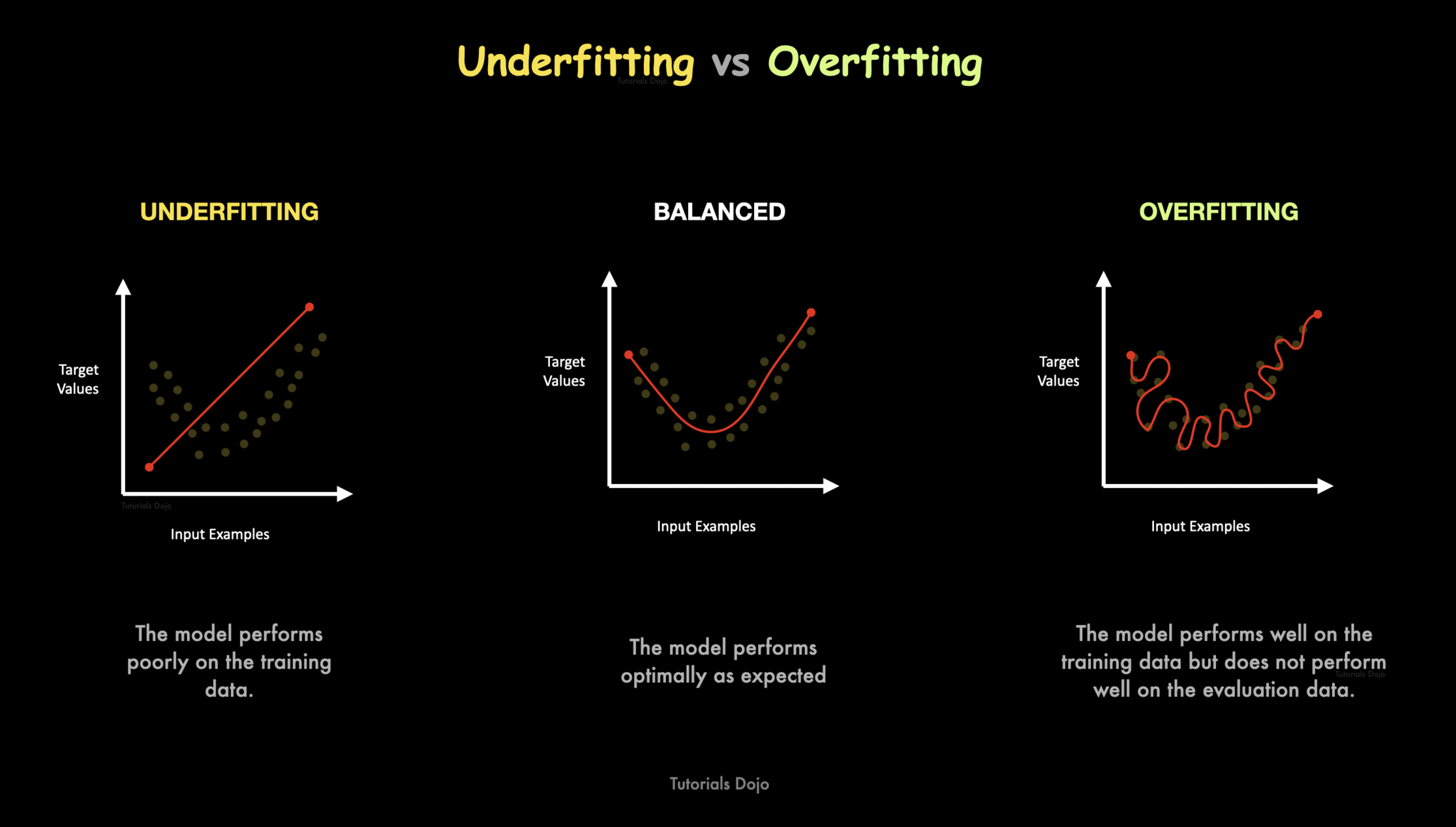
Underfitting
- When the does not capture the underlying patterns in the data.
- Generally occurs if the model is too simple.
- Performs poorly on the training set
Overfitting
- When the model memorizes the training data set.
- The data available may not be sufficient or the model is too complex.
- This leads to model performing poorly on test data / unseen data.
- The model is not able to generalize.
Regularization
- It is used to prevent overfitting be restricting model’s complexity.
- It reduces large weights and improves generalization.
- It achieves so by adding penalties to the loss function or introducing random noise during training.
L1 Regularization (Lasso)
- adds the sum of the absolute values of the weights to the loss function.
loss = loss_og + lambda * sum(abs(w) for w in weights)- it tends to produce sparse models where many weights become exactly zero
- effectively performing feature selection
lambda: hyperparameter controlling regularization strength
L2 Regularization (Ridge)
- also called Weight decay
- adds the sum of the squared values of the weights to the loss function.
loss = loss_og + lambda * sum(w^2 for w in weights)- it penalizes large weights and tends to produce models with many small weights rather than a few large ones.
optimizer = torch.optim.Adam(model.parameters(), lr=0.001, weight_decay=1e-5)- It can also be applied directly using
weight_decay(lamda or regularization strength).
- It can also be applied directly using
PyTorch implementation
def train_with_regularization(model, train_loader, optimizer, criterion, l1_lambda=0.0, l2_lambda=0.0):
    model.train()
    for inputs, targets in train_loader:
        optimizer.zero_grad()
        outputs = model(inputs)

        # Original loss
        loss = criterion(outputs, targets)

        # L1 regularization
        if l1_lambda > 0:   # skip the regularixation if lambda = 0, thus saving computation
            l1_reg = torch.tensor(0., requires_grad=True)
            for param in model.parameters():
                l1_reg = l1_reg + torch.sum(torch.abs(param))
            loss = loss + l1_lambda * l1_reg

        # L2 regularization
        if l2_lambda > 0:
            l2_reg = torch.tensor(0., requires_grad=True)
            for param in model.parameters():
                l2_reg = l2_reg + torch.sum(param ** 2)
            loss = loss + l2_lambda * l2_reg

        loss.backward()
        optimizer.step()
Dropout
- randomly deactivates a fraction of neurons during each training iteration.
- prevents neurons from co-adapting too much.
- forces the model to learn robust features.
Working
- During Training:
- Some neurons are randomly turned off (set to zero) with probability
r(drop rate). - This prevents the network from relying too much on specific neurons and helps it learn more general features.
- Some neurons are randomly turned off (set to zero) with probability
- During Inference (Testing):
- All neurons are used, but their outputs are scaled by
p = 1 - r(keep probability). - This ensures that the total activation remains similar to training, avoiding unexpected behavior.
- All neurons are used, but their outputs are scaled by
Let there be an activation tensor with 4 neurons :
[2, 4, 6, 8]r = 0.5andp = 0.5- During training
- half the neurons are turned off
[2, 0, 6, 0]- During Inference
- All the neurons are used and scaled by
p = 0.5
[1, 2, 3, 4]
- drop rate (
r)
- fraction of neurons dropped / set to 0.
- keep probability (
p)
- fraction of neurons that remain active during training
p = 1-r
PyTorch implementation
class SimpleNetWithDropout(nn.Module):
    def __init__(self, input_size, hidden_size, output_size, dropout_rate=0.5):
        super(SimpleNetWithDropout, self).__init__()
        self.fc1 = nn.Linear(input_size, hidden_size)
        self.dropout = nn.Dropout(dropout_rate)  # Dropout layer
        self.relu = nn.ReLU()
        self.fc2 = nn.Linear(hidden_size, output_size)

    def forward(self, x):
        x = self.fc1(x)
        x = self.relu(x)
        x = self.dropout(x)  # Apply dropout after activation
        x = self.fc2(x)
        return x
- Typical dropout rates range from
0.2 to 0.5. - Dropout is usually applied after activation functions.
- Modern frameworks handle the scaling during inference automatically.
Early Stopping
- stops training when the performance on a validation set starts to degrade, indicating that the model is beginning to overfit.
- It requires a validation set to function.
PyTorch implementation
def train_with_early_stopping(model, train_loader, val_loader, optimizer, criterion, patience=5, max_epochs=100):
    best_val_loss = float('inf')
    counter = 0

    for epoch in range(max_epochs):
        # Train for one epoch
        train_loss = train_one_epoch(model, train_loader, optimizer, criterion)

        # Evaluate on validation set
        val_loss = evaluate(model, val_loader, criterion)

        print(f"Epoch {epoch+1}/{max_epochs}, Train Loss: {train_loss:.4f}, Val Loss: {val_loss:.4f}")

        # Check if validation loss improved
        if val_loss < best_val_loss:
            best_val_loss = val_loss
            counter = 0
            # Save the best model
            torch.save(model.state_dict(), 'best_model.pt')
        else:
            counter += 1

        # Check if we should stop early
        if counter >= patience:
            print(f"Early stopping triggered after {epoch+1} epochs")
            break

    # Load the best model
    model.load_state_dict(torch.load('best_model.pt'))
    return model
- after each epoch it checks if the validation loss improved or not
- if improved
- Saves the current model as the best model
- if did not improved
- Increases a
countervariable which may cause early exit if the number of times this happens increases a fixed variablepatience.
- Increases a
- if improved
Normalization
- Normalization methods standardize inputs or intermediate outputs to stabilize and speed up training.
- Stabilizes training by keeping activations well scaled.
- Ensures that data distributions remain stable.
- Speeds up convergence, prevents gradient issues.
- the input layer distribution is constantly changing due to weight update. In this case, the following layer always needs to adapt to the new distribution. It causes slower convergence and unstable training
- It is different from normalization done during preprocessing
- It happens during data preparation even before the data enters the network.
- Applied once to the entire dataset.
- Makes features comparable in scale.
- This normalization occurs during training.
- integrated into the architecture.
- applied at each forward pass.
- stabilizes and accelerates training.
Batch Normalization
- normalizes the activations of each layer for each mini-batch,
- helps address internal covariate shift
- allows for higher learning rates.
Working
- Normalize activations to have zero mean and unit variance.
- Scale and shift with learnable parameters (gamma and beta).
- Keep running statistics during training for use during inference.
- Applying learnable scale and shift parameters: \(y = \gamma \hat{x} + \beta\)
PyTorch implementation
self.bn = nn.BatchNorm1d(num_features)
class ConvNetWithBatchNorm(nn.Module):
    def __init__(self):
        super(ConvNetWithBatchNorm, self).__init__()
        self.conv1 = nn.Conv2d(3, 16, kernel_size=3, padding=1)
        self.bn1 = nn.BatchNorm2d(16)  # BatchNorm after conv layer
        self.relu = nn.ReLU()
        self.pool = nn.MaxPool2d(2, 2)
        self.fc = nn.Linear(16 * 16 * 16, 10)

    def forward(self, x):
        x = self.conv1(x)
        x = self.bn1(x)  # Apply batch norm before activation
        x = self.relu(x)
        x = self.pool(x)
        x = x.view(-1, 16 * 16 * 16)
        x = self.fc(x)
        return x
- Typically applied before activation functions.
- Also serves as regularization technique.
Layer Normalization
- normalizes activations per sample instead of across the batch.
- normalizes across all features for each example independently, making it effective for recurrent networks and transformers where batch statistics may vary significantly.
PyTorch implementation
self.ln = nn.LayerNorm(normalized_shape)
import torch.nn as nn

class RNNWithLayerNorm(nn.Module):
    def __init__(self, input_size, hidden_size, output_size):
        super(RNNWithLayerNorm, self).__init__()
        self.rnn = nn.LSTM(input_size, hidden_size, batch_first=True)
        self.ln = nn.LayerNorm(hidden_size)  # Layer normalization
        self.fc = nn.Linear(hidden_size, output_size)

    def forward(self, x):
        output, _ = self.rnn(x)
        output = self.ln(output)  # Apply layer norm
        output = self.fc(output[:, -1, :])  # Use only the last output
        return output
Instance Normalization
- Instance normalization normalizes each sample individually, often used in style transfer tasks.
- Computes mean and variance for each sample and each channel.
self.inorm = nn.InstanceNorm2d(num_features)
Group Normalization
- Group normalization divides channels into groups and normalizes within them
- Splits channels into groups and computes mean and variance for each group.
self.gn = nn.GroupNorm(num_groups, num_channels)
Technique Combinations
- Different regularization and normalization techniques can be combined for better results:
- BatchNorm + Dropout: Apply dropout after batch normalization, not before
- L2 + Dropout: These work well together and address different aspects of overfitting
- Early Stopping + L2: Provides complementary benefits