3. Computer Vision: Transfer Learning
Transfer Learning
- Training deep learning models from scratch requires massive amounts of data and computational resources.
- Transfer learning allows to use pre-trained models, which have already learned useful features from large datasets like ImageNet.
- It is a technique where a model trained on one task is reused for another related task.
- Instead of training from scratch, we use a pre-trained model and perform either:
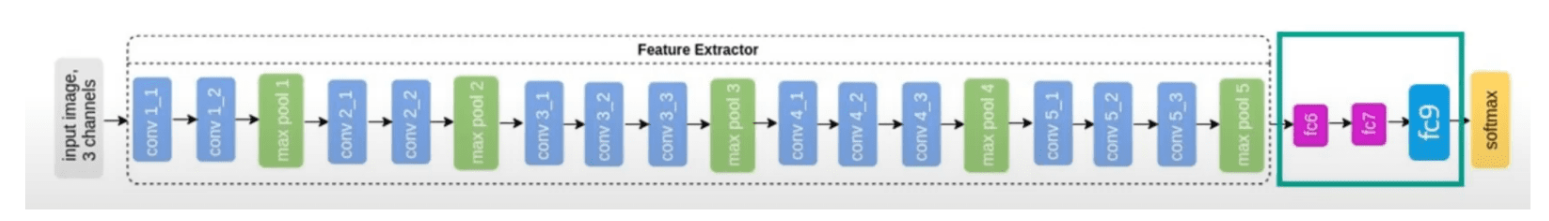
- Feature Extraction: Freeze the pre-trained model’s weights and use it as a feature extractor.
- Fine-Tuning: Unfreeze some or all layers and train the model further on new data.
Feature Extraction
- Use pretrained feature extractor.
- Modify the classifier to suit new dataset.
- The pre-trained ImageNet Feature Extractor has learned valuable features for detecting many different object types.
- Assume such features are general enough that we only need to re-train the classifier portion of the network.
Some image trasformations
-
transforms.RandomResizedCrop(size = 256, scale =(0.8, 1.0))- randomly crops the image to a fixed size (256x256 pixels).
- scaling factor (0.8, 1.0) means the cropped region will be between 80% to 100% of the original image’s size.
-
transforms.RandomRotation(degrees=15)- rotates the image by a random angle in the range [-15, +15] degrees.
- makes the model more robust to different orientations
-
transforms.RandomHorizontalFlip()- flips the image horizontally (left ↔ right) with a probability of 0.5.
- thus the model will generalize better by making it invariant to horizontal flips.
-
transforms.CenterCrop(size=224)- crops the central 224x224 region from the image.
-
transforms.ToTensor()- converts PIL image (NumPy array) to PyTorch Tensor.
- scales the pixel values from [0, 255] (unit8) to [0, 1] (float32).
-
transforms.Normalize([0.485, 0.456, 0.406], [0.229, 0.224, 0.225])- normalizes the image using the mean and standard deviation values of the ImageNet dataset.
Load the dataset and freeze all the layers
model = models.resnet50(weights='DEFAULT')
model = model.to(device)
for param in model.parameters():
    pqram.requires_grad = False
Unfreeze the final layer of the classifier’s head
Information about all the layers of the model can be found out using
print(model)
fc_inputs = model.fc.in_features

model   .fc = nn.Sequential(
    nn.Linear(fc_inputs, 256),  # Fully connected layer with 256 neurons
    nn.ReLU(),  # Apply ReLU activation
    nn.Dropout(0.4),  # Apply dropout with 40% probability to prevent overfitting
    nn.Linear(256, num_classes),  # Output layer with number of classes as output neurons
    nn.LogSoftmax(dim=1)  # Apply LogSoftmax for multi-class classification (used with Negative Log Likelihood Loss)

    model.to(device)
)
- Define a new fully connected layer with custom architecture for classification.
nn.Sequential: used to stack layers in neural network in the given order.
Configuring the training
criterion = nn.NLLLoss()
lr = 0.01

optimizer = optim.SGD(params = model.parameters(), lr = lr, momentum = 0.9)
Training
- The model can be now be trained like any other model.
- There is also another way to train by validating the model using validation dataset at each epoch.
Train & Validate
This is a pseudocode.
def train_and_validate(model, loss_fn, optimizer, epochs):
    best_loss = 100000.0 # very high number

    for epoch in range(epochs):
        print("Epoch: {}/{}".format(epoch+1, epochs))

        # Training Phase
        model.train()
        train_loss, train_acc = 0, 0

        for inputs, labels in train_loader:
            inputs = imputs.to(device)
            labels = labels.to(device)

            optimizer.zero_grad()
            outputs = model(inputs)
            loss = criterion(outputs, labels)
            loss.backward()
            optimizer.step()

            train_loss += loss * batch_size
            train_acc += correct_predictions(outputs, labels)

        # Validation Phase
        model.eval()
        valid_loss, valid_acc = 0, 0

        with no_grad():
            for inputs, labels in valid_loader:
                inputs = imputs.to(device)
                labels = labels.to(device)
                outputs = model(inputs)
                loss = criterion(outputs, labels)

                valid_loss += loss * batch_size
                valid_acc += correct_predictions(outputs, labels)

        # Save best model
        if valid_loss < best_loss:
            best_loss = valid_loss
            save_model(model, "best_model.pt")

        # Print epoch summary
        print_metrics(epoch, train_loss, train_acc, valid_loss, valid_acc)

    return model
- Alternates between training & validation.
- Tracks loss & accuracy for both phases.
- Saves the best model based on validation loss.
- Optimized with gradient updates during training.
Colab Notebook with the complete implementation can be accessed here
Therefore transfer learning / feature extraction is performed by retaining most of the pre-trained model and only replace the final classification layer to classify a smaller subset of categories (e.g., a few out of ImageNet’s 1,000 classes).
The earlier layers (convolutional layers) remain frozen since they already learned general feature representations (edges, textures, shapes, etc.).