Object Detection , R-CNN, Fast R-CNN & Faster R-CNN

The input to the model is an image, and the output is an array of bounding boxes, and a class label for every bounding box.
There can be multiple objects in the image and thr task may be to identify and locate them in the image.

Image Classification : single class label for the entire image

Segmentation : class label for every pixel

Object Detection : class label and bounding box for each object in the image

Sliding Window Approach

Input image is split into multiple crops and each crop of the image is classified and if the crop contains a class, then the crop is decided as the bounding box.
One of the oldest approach.
Not used in practice as each input may have 1000s of crops.

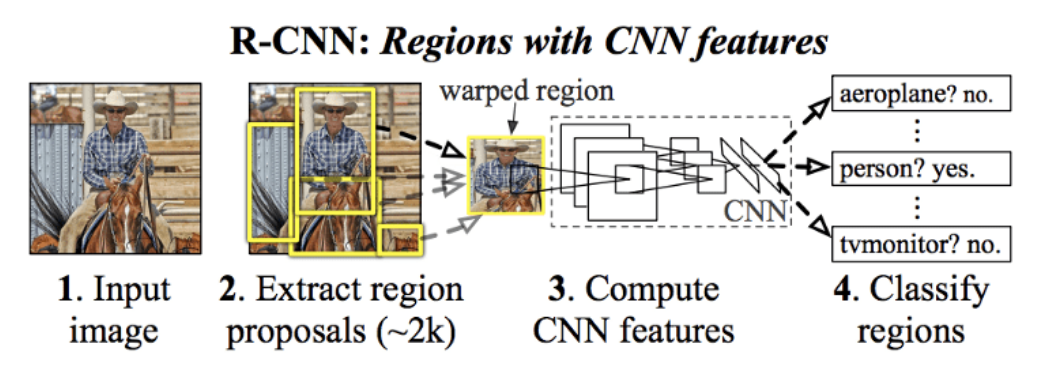
R-CNN

Region-based Convolutional Neural Network
Divides the object detection task into 2 stages :
1. Region proposal
2. Onject Classification
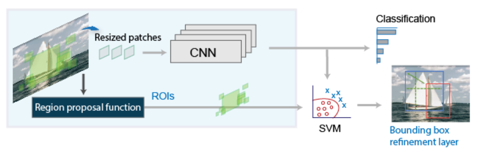
R-CNN workflow consists of 4 steps :
- Region Proposal Generation
  - Genrate approx 2000 region proposals per image using the Selective Search algo.
  - These proposals serve to identify potential areas within an image that are likely to contain objects, thereby focusing the subsequent computational resources on the most relevant parts of the image rather than exhaustively searching the entire image.
  - Selective Search :
    - It is a greedy hierarchial (bottom up) clustering approach
      1. Over-segmenting the image into small regions.
      2. Then merging similar regions step by step to form larger ones.
      3. Collecting all regions seen during the process as region proposals.
    - combines similar regions based on texture, color, and other visual cues to identify potential object locations.
- Feature Extraction
  - Each proposed region is resized to a fixed dimension (commonly 224×224 pixels) and passed through a pre-trained CNN to extract high-dimensional feature representations.
- Object Classification
  - The extracted feature vectors are fed into a set of class-specific SVMs, where each SVM determines whether the region contains an object of a particular class.
- Bounding Box Regression
  - adjusts the coordinates of the proposed regions to better align with the actual object boundaries.

Mathematics of R-CNN

Let the proposal box from selective search be :
- \[P = (x_p, y_p, w_p, h_p)\]
  - xp , yp : center of the proposal bax
  - wp, hp : width and height
Ground truth box :
- G = (x, y, w, h)

Want the model to learn how to adjust the proposal to get the ground truth box.

Want the model to predict how much to shift and scale the proposal — in a way that works for boxes of all sizes.

Compute the regression targets (how much the proposal should shift and scale to become the ground truth)
- \(t_x = \frac{x - x_p}{w_p}\) (horizontal shift, normalized)
- \(t_y = \frac{y - y_p}{h_p}\) (vertical shift, normalized)
- \(t_w = \log ( \frac{w}{w_p} )\) (how much to scale the width)
- \(t_h = \log ( \frac{h}{h_p} )\) (how much to scale the height)

During training

Predict offsets
- Pass the proposal features through a regression head (a few fully connected layers) in neural network.
- It outputs predicted deltas for each proposal:
  - t̂ = model(proposal_features) → [t̂x, t̂y, t̂w, t̂h]
Calculate Loss (Smooth L1 Loss)
- \[\mathcal{L}_{\text{reg}} = \sum_{i \in \{x, y, w, h\}} \text{SmoothL1}(\hat{t}_i - t_i)\]
- \[\text{SmoothL1}(x) = \begin{cases} 0.5 \, x^2 / \beta, & \text{if } |x| < \beta \\ |x| - 0.5 \beta, & \text{otherwise} \end{cases}\]
- where x = t̂i - ti
- \(\beta\) is a threshold (usually = 1)
  - controls the transition between L2 loss (quadratic) and L1 loss (linear).
Backpropagate
- combine this regression loss with the classification loss (e.g. softmax for object classes), and backpropagate to train the model:
  - \(L = L_{cls} + \lambda \cdot L_{reg}\)

During inference

Apply the predicted set of deltas to the proposal boxes
- \(x = t^x \cdot w_p + x_p\)
- \(y = t^y \cdot h_p + y_p\)
- \(w = w_p \cdot \exp(t^w)\)
- \(h = h_p \cdot \exp(t^h)\)
This gives refined bounding box that better fits the object.
Pass to Non-Maximum Suppression (NMS) to remove duplicates
- suppressing the weaker bounding boxes based on their overlap with stronger ones (usually using the Intersection over Union, IoU, metric).

Fast R-CNN

Problems with R-CNN

Slow training : Multiple stages (feature extraction + SVM training + bounding box regression)
Slow testing : Each region proposal is passed through CNN independently.
No end-to-end learning : CNN does not update weights during SVM training.

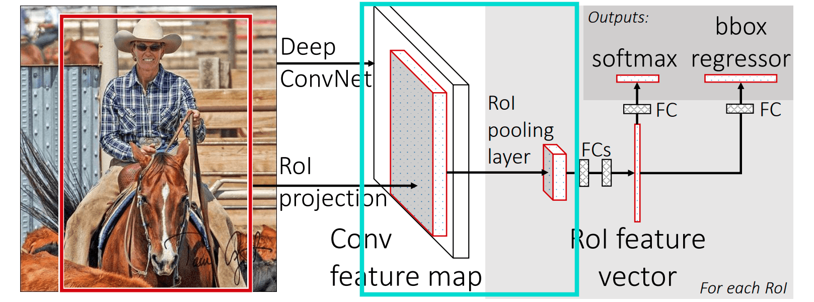
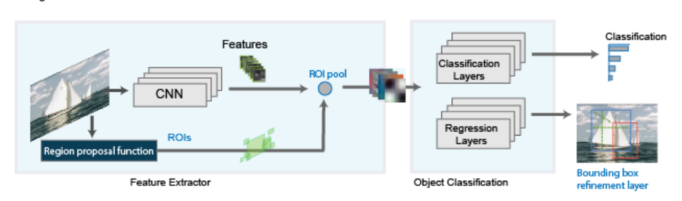
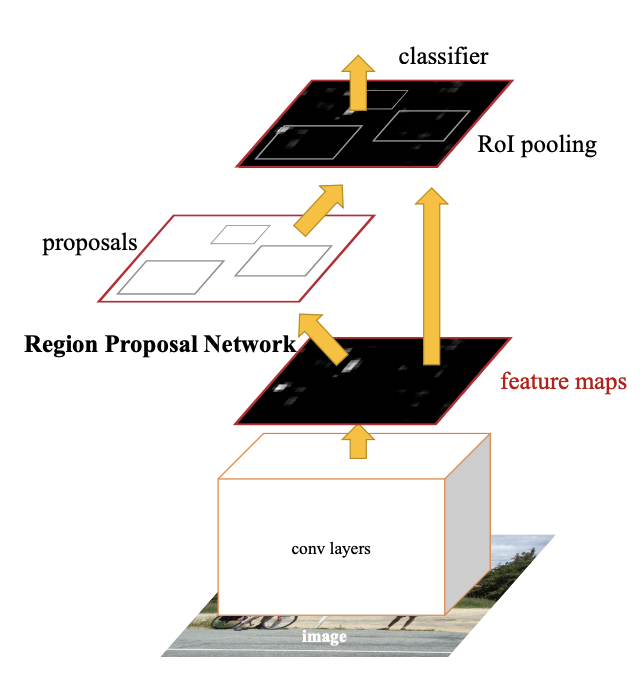
Fast R-CNN pipeline

Processing the entire image only once with a CNN.
Using Region of Interest (RoI) pooling on the feature map to extract fixed-length feature vectors.
Training classification and bounding box regression jointly in one forward pass.

Steps in Fast R-CNN

Input : An image and a list of region proposals (e.g., from Selective Search).
Convolutional Layer : Feed the image into a CNN to get a convolutional feature map.
RoI Pooling : For each RoI, extract a fixed-size feature vector from the feature map.
Fully Connected Layers : Pass RoI feature vectors through FC layers.
Output Layers :
- A softmax classifier (multi-class + background)
- A bounding box regressor for each class.

Region of Interest (RoI) Pooling

Allows the network to take region proposals of different sizes and convert them into fixed-size feature maps.
The model generates proposals of different sizes.
To process these proposals using fully connected layers, they need to be converted into fixed (uniform) sizes (eg. 7 x 7).
RoI Pooling fixes this mismatch by “compressing” each RoI into a fixed-size grid, while preserving spatial information.
Steps of RoI Pooling
- Given :
  - A feature map (output of a CNN).
  - A region proposal (RoI) (eg. a rectangle on that feature map).
    - (r, c, h, w) that indicates its top-left corner (r, c) and its height and width (h, w).
  - Pool this RoI into a fixed-size output, e.g., 7×7.
- Steps :
  1. Map RoI to the feature map
    - The RoIs are originally in image coordinates.
    - They are scaled to match the feature map size (since the CNN downscales the input).
  2. Divide RoI into grid cells
    - If we want to pool into H×W (e.g., 7×7).
    - The RoI is divided into H×W bins (equal or nearly equal in size).
  3. Max Pooling
    - For each bin, perform max pooling over the corresponding patch in the feature map.
Result : A fixed-size feature map for that RoI.

bins : small rectangular region (or sub-window) inside a Region of Interest (RoI).

Example :
An RoI of 14 pixels × 14 pixels on the feature map.

Want to pool it to 7×7.

want 7 rows and 7 columns → total 7×7 = 49 bins.

Since original RoI is 14×14, and you want 7 rows and 7 columns:

Each bin must cover:

height of bin = \(\frac{14}{7} = 2 \, pixels (vertical)\)

height of bin = \(\frac{14}{7} = 2 \, pixels (horizontal)\)
So each bin is a small 2×2 patch.
----------------------------------
| 2x2 | 2x2 | 2x2 | ... | 2x2 | 2x2 |
| 2x2 | 2x2 | 2x2 | ... | 2x2 | 2x2 |
| 2x2 | 2x2 | 2x2 | ... | 2x2 | 2x2 |
| ...                               |
| 2x2 | 2x2 | 2x2 | ... | 2x2 | 2x2 |
----------------------------------
Inside each 2×2 bin:

Pick the maximum value among the 4 numbers (2×2 = 4 numbers).

This gives one single value.

Thus we will get 7×7 feature map.

Mathematically
- \(R = [x_1, y_1, x_2, y_2]\) is a region on the feature map.
- Output size = H x W.
- Each bin covers :
  - \[h_{bin} = \frac{y_2 - y_1}{H} , \quad w_{bin} = \frac{x_2 - x_1}{W}\]
- For each bin apply,
  - \[output_{i,j} = max\]
  - \[\text{output}_{i,j} = \max_{(x, y) \in \text{bin}(i, j)} \text{features}(x, y)\]
The 7×7 pooled feature map (from each RoI) is flattened into a 1D vector.
The flattened vector is passed through fully connected layers.
- They help to learn higher-level features from RoI.
After the FC layers, the network splits into two heads:

Branch	Purpose	Output
Classifier head	Classify the object	Probability distribution over all classes + 1 background class
Bounding box regressor head	Fine-tune box coordinates	4 numbers (dx, dy, dw, dh) per class

Loss Function of Fast R-CNN

Fast R-CNN uses a multi-task loss, one part for classification and one part for bounding box regression.

\[L(p,u,t,v) = L_{cls}(p,u) + \lambda[u \geq 1] L_{loc}(t,v)\]

p = predicted class probabilities (output from softmax).
u = true class label (integer; 0 = background, 1 = first object class, etc.).
t = predicted bounding box offsets.
v = true bounding box regression targets.
λ = balance weight (usually set to 1).
[u≥1] = indicator function → only apply bounding box loss if the RoI is not background.
\(L_{cls}\) : Classification loss
- \[L_{cls}(p,u) = -log p_u\]
- pu is the probability the model assigned to the correct class u.
- u = 0 means the RoI is background
Localisation Loss
- Smooth L1 loss applied on the bounding box coordinates.
- only computed when RoI is foreground.

Faster R-CNN

Uses Region Proposal Network (RPN) to generate proposals instead of Selective search.
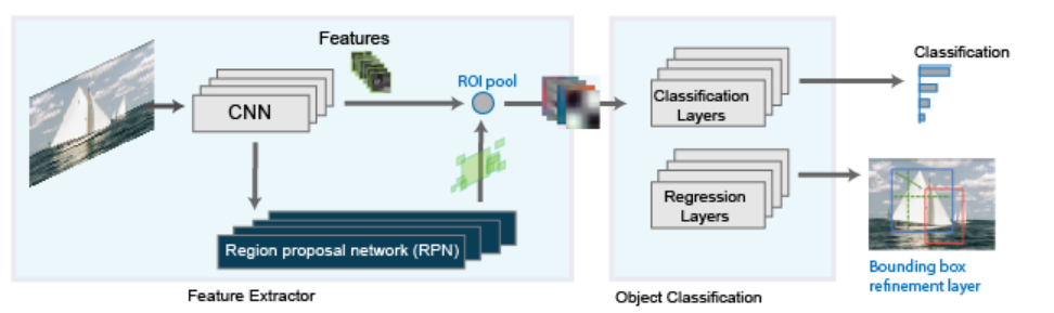
Faster R-CNN = Feature extractor + Region Proposal Network (RPN) + Fast R-CNN head

Steps :

Input Image → Pass through a Convolutional Neural Network (e.g., ResNet, VGG) → get a feature map.
Region Proposal Network (RPN) :
- Slides a small network over the feature map.
- At each location, proposes possible object bounding boxes (called anchors).
RoI Pooling :
- Takes these proposals and extracts fixed-size feature vectors (Regions of Interest) from the feature map.
Classification and Regression:
- A fully connected head predicts:
  - Class scores (object category)
  - Bounding box refinements

Region Proposal Networks (RPN)

It is a small neural network which slides over the CNN feature map.
It predicts for every location :
- Whether an object exists (objectness score).
- How to adjust a default box (anchor) to better fit the object (bounding box regression).

Steps :

Take feature map from CNN (size W×H×C).
Place anchors at every location (pixel) in the feature map:
- Anchor are pre-defined boxes of different sizes and shapes placed over points on the feature map.
- Multiple anchors are used per location — to cover different sizes and aspect ratios.
For each anchor, predict:
- A binary classification:
  - Is the anchor a foreground (object) [Positive anchor] or background (non-object) [Negative anchor]?
- A bounding box regression:
  - How to move and resize this anchor to better fit the object.

RPN Training :

Label anchors
- Positive Anchors :
  - Anchors that have highest IoU with a ground-truth box
  - OR anchors whose IoU > 0.7 with any ground-truth box
- Negative Anchors :
  - Anchors whose IoU < 0.3 with all ground-truth boxes

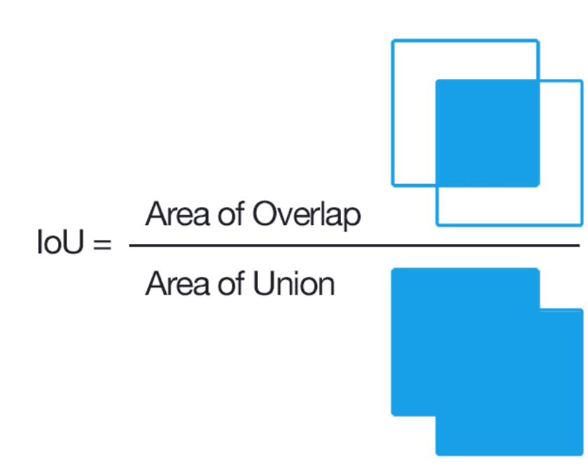
IoU = Intersection over Union

It is an evaluation metric used to measure the accuracy of an object detector on a particular dataset.

RPN Loss

\[L(p_i,t_i) = \frac{1}{N_{cls}} \sum_i L_{cls}(p_i,p_i ^*) + \lambda \frac{1}{N_{reg}} \sum_i p_i ^* L_{reg} (t_i, t_i ^*)\]

\(p_i\) = predicted objectness probability (is there an object or not?) for anchor
\(p_i ^*\) = ground-truth label for anchor (1 if anchor is positive, 0 if negative)
\(t_i\) = predicted box regression parameters (how much to move/resize anchor)
\(t_i ^*\) = ground-truth box regression targets (true adjustments)
\(N_{cls}\) = Number of anchors used for classification loss calculation = number of all sampled anchors (both positives + negatives)
\(N_{reg}\) = Number of anchors used for regression (bounding box adjustment) loss calculation = number of positive anchors only (because regression is meaningful only for positives)
\(L_{cls}\) = log loss over 2 classes (object / not object)
\(L_{reg}\) = smooth L1 loss between predicted and ground-truth box
λ = balancing factor between classification and regression

Input image is passed through a CNN backbone and a feature map is obtained.
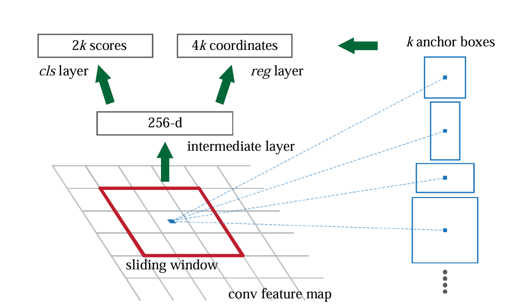
A small sliding window (3x3) slides over every spatial location.
At each sliding window location, we want to propose several bounding boxes.
For each window location, apply a small network (3x3 conv) producing a 256-dimensional feature vector.
- This is called Intermediate Layer or 256-d.
At each location, place k predefined anchor boxes of different scales and aspect ratios.
- if k=9:
  - 3 scales (small, medium, large)
  - 3 aspect ratios (tall, wide, square)
  - Thus, 9 anchors at every single feature map point.
From the 256-d intermediate feature:
- A cls layer predicts 2 scores per anchor (is anchor object or background)
- A reg layer predicts 4 coordinates per anchor (how much to move/resize this anchor to better fit the object)
Since there are k anchors at each location:
- 2k scores (for classification)
- 4k coordinates (for regression)
Use the predicted bbox (bounded box) regressions to adjust the anchor boxes into proposals (slightly shifted, resized anchors).
- Apply NMS (Non-Maximum Suppression) : Remove overlapping boxes that have high Intersection-over-Union (IoU), keeping only best ones.
Rest same as Fast R-CNN

Object Detection using PyTorch

Importing the model

model = torchvision.models.detection.fasterrcnn_resnet50_fpn(
    weights=torchvision.models.detection.FasterRCNN_ResNet50_FPN_Weights.DEFAULT
)
model.eval()

Class labels and Giving colour to each label

COCO_INSTANCE_CATEGORY_NAMES = [    # list of labels (mapping numbers to names).
    '__background__', 'person', 'bicycle', 'car', 'motorcycle', 'airplane', 'bus',
    'train', 'truck', 'boat', 'traffic light', 'fire hydrant', 'N/A', 'stop sign',
    'parking meter', 'bench', 'bird', 'cat', 'dog', 'horse', 'sheep', 'cow',
    'elephant', 'bear', 'zebra', 'giraffe', 'N/A', 'backpack', 'umbrella', 'N/A', 'N/A',
    'handbag', 'tie', 'suitcase', 'frisbee', 'skis', 'snowboard', 'sports ball',
    'kite', 'baseball bat', 'baseball glove', 'skateboard', 'surfboard', 'tennis racket',
    'bottle', 'N/A', 'wine glass', 'cup', 'fork', 'knife', 'spoon', 'bowl',
    'banana', 'apple', 'sandwich', 'orange', 'broccoli', 'carrot', 'hot dog', 'pizza',
    'donut', 'cake', 'chair', 'couch', 'potted plant', 'bed', 'N/A', 'dining table',
    'N/A', 'N/A', 'toilet', 'N/A', 'tv', 'laptop', 'mouse', 'remote', 'keyboard', 'cell phone',
    'microwave', 'oven', 'toaster', 'sink', 'refrigerator', 'N/A', 'book',
    'clock', 'vase', 'scissors', 'teddy bear', 'hair drier', 'toothbrush'
]

COLORS = np.random.uniform(0, 255, size=(len(COCO_INSTANCE_CATEGORY_NAMES), 3)) # assigns random color to each label

Prediction function

def get_prediction(img_path, threshold):
  img = Image.open(img_path)
  transform = T.ToTensor()
  img = transform(img)

  pred = model([img])

  pred_data = pred[0]

  labels = pred_data['labels'].detach().cpu().numpy()
  boxes = pred_data['boxes'].detach().cpu().numpy()
  scores = pred_data['scores'].detach().cpu().numpy()

  valid_indices = scores > threshold

  pred_boxes = [((b[0], b[1]), (b[2], b[3])) for b in boxes[valid_indices]]
  pred_class = [COCO_INSTANCE_CATEGORY_NAMES[i] for i in labels[valid_indices]]

  return pred_boxes, pred_class

threshold : only keep predictions with a confidence score higher than this value.
pred = model([img])
- pass the image as a list because most models expect a batch (even of size = 1)
- pred is the model’s raw output — usually a list of dictionaries where each dictionary contains:
  - boxes : bounding box coordinates
  - labels : predicted class indices
  - scores : confidence scores for each prediction
pred[0] : because the batch size is 1 (only one image).
valid_indices = scores > threshold
- creates a boolean array: True for scores greater than threshold, otherwise False.
For each valid prediction :
- pred_boxes = [((b[0], b[1]), (b[2], b[3])) for b in boxes[valid_indices]]
  - Save the bounding box in the format ((x1, y1), (x2, y2)).
- pred_class = [COCO_INSTANCE_CATEGORY_NAMES[i] for i in labels[valid_indices]]
  - Convert the class index to human-readable class name.

Using OpenCV for plotting boxes

def object_detection(img_path, threshold):
  boxes, pred_cls = get_prediction(img_path, threshold)

  img = cv2.imread(img_path)
  img = cv2.cvtColor(img, cv2.COLOR_BGR2RGB)
  
  rect_th = max(round(sum(img.shape) / 2 * 0.003), 2)   #thickness for drawing bounding boxes based on image size
  text_th = max(rect_th - 1, 1) # annotation thickness

  for i in range(len(boxes)):
     # Extract bounding box coordinates from the prediction output
    p1, p2 = (int(boxes[i][0][0]), int(boxes[i][0][1])), (int(boxes[i][1][0]), int(boxes[i][1][1]))

    color = COLORS[COCO_INSTANCE_CATEGORY_NAMES.index(pred_cls[i])]

    cv2.rectangle(
        img,
        p1, # top left corner
        p2, # bottom right corner
        color = color, # bbox color
        thickness=rect_th # line thickness
    )

    w, h = cv2.getTextSize(
            pred_cls[i],  # Object class name
            0,  # Font face
            fontScale=rect_th / 3,  # Scale font relative to box thickness
            thickness=text_th  # Text thickness
        )[0] 

    # Determine if text label should be placed inside or outside the bounding box
    outside = p1[1] - h >= 3  # Check if there is enough space to put text above the box
    # Calculate coordinates for the background rectangle that holds the text
    p2 = p1[0] + w, p1[1] - h - 3 if outside else p1[1] + h + 3

    cv2.rectangle(
        img,
        p1,
        p2,
        color=color,
        thickness=-1, # Draw a filled rectangle for the class label background
        lineType=cv2.LINE_AA
    )

    cv2.putText(
            img,
            pred_cls[i],  # Class name
            (p1[0], p1[1] - 5 if outside else p1[1] + h + 2),  # Adjust text position
            cv2.FONT_HERSHEY_SIMPLEX,  # Font type
            rect_th / 3,  # Scale font size
            (255, 255, 255),  # White text color
            thickness=text_th + 1  # Text thickness
        )
  plt.figure(figsize=(15,12))
  plt.imshow(img)
  plt.xticks([])
  plt.yticks([])
  plt.show()

Performing Object detection

object_detection('path', threshold=0.8)

Colab Notebook with the complete implementation can be accessed here

Object Detection , R-CNN, Fast R-CNN & Faster R-CNN

Sliding Window Approach

R-CNN

Region Proposal Generation

Feature Extraction

Object Classification

Bounding Box Regression

Mathematics of R-CNN

During training

Predict offsets

Calculate Loss (Smooth L1 Loss)

Backpropagate

During inference

Fast R-CNN

Problems with R-CNN

Fast R-CNN pipeline

Steps in Fast R-CNN

Region of Interest (RoI) Pooling

Steps of RoI Pooling

Map RoI to the feature map

Divide RoI into grid cells

Max Pooling

Mathematically

Loss Function of Fast R-CNN

\(L_{cls}\) : Classification loss

Localisation Loss

Faster R-CNN

Steps :

Region Proposal Networks (RPN)

Steps :

RPN Training :

RPN Loss

Object Detection using PyTorch

Importing the model

Class labels and Giving colour to each label

Prediction function

Using OpenCV for plotting boxes

Performing Object detection