1. NLP: Recurrent Neural Networks [RNN]

RNNs

• Process Sequential Data.
  • Data in which :
    1. Order of elements matter.
    2. Each element depends on the prevous element.
• The output at one time step is fed back into the network at the next time step
  • Thus, it is called recurrent.
• Share the same parameters / weights across all time steps.

• They have a memeory which captures information about what has been calculated so far.

• 

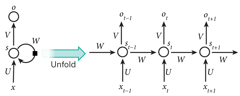
Breakdown of RNN

• x_t : input at time step t.
  • It can be a one-hot vector encoding.
• s_t : Hidden state at time t.
  • It is the memory component of the RNN.
  • Calculated based on the previous hidden state and the current step’s input.
  • It is calculated as : \(s_t = f(U x_t + W s_{t-1})\)
    • f : nonlinearity (eg. ReLU or Tanh).
  • s_t-1 : required to calculate the first hidden state.
    • Can be all zeros initially.
• o_t : output at time step t
  • Vector of probabilities : \(o_t = softmax(V s_t)\)

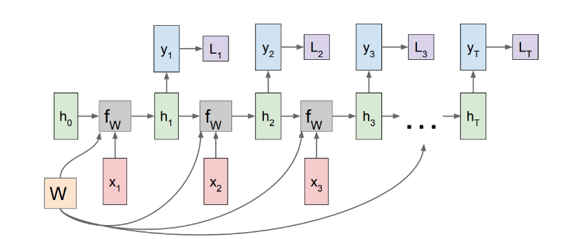
Training RNN / BBPT

• Algorithm used is Backpropagation Through Time (BPTT).
  • Apply chain rule to propagatethe error backward through time, consdering the influence of each timestep’s calculations on the final loss.
• RNN processes a sequence of inputs \(x_1,x_2,...,x_T\).
• At each timestep t, the network performs the following calculations :

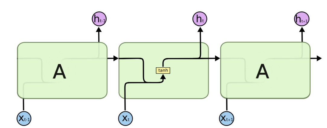
• Linear transformation of current input (x_t) and prevous hidden state (s_t-1) to give pre-activation : \(z_t = U x_t + W s_{t-1}\)
• Pre-activation is passed through non-linearity to produce current hidden state : \(s_t = tanh(z_t)\)
• Linear transformation of current hidden state to produce output logits : \(o_t = V s_t\)
• Obtain probability distribution over the output classes : \(p_t = softmax(y_t)\)
• Loss calculation : \(J_t = crossentropy(p_t, labels_t)\)

• J_t = Total Cost of a given sequence of inputs = \(- \sum\limits_{i} (labels)_{t,i} \log(p_{t,i})\)
• U : weight matrix for input-to-hidden connection.
• V : weight matrix for hidden-to-output connection.

• W : weight matrix for recurrent hidden-to-hidden connection.

• The total loss for a sequence of length T is the sum of the losses at each timestep : \(J = \sum\limits_{t=1}^{T} J_t\)

• Goal of BPTT : Minimize the total loss J by adjusting the parameters U, W, and V using gradient descent by calculating the gradients of J wrt these parameters.
• These gradients are computed by applying the chain rule through the unrolled RNN structure over time.

• 

Gradient w.r.t V

• \[\frac {\partial J_t}{\partial V} = \frac {\partial J_t}{\partial o_t} \frac {\partial o_t}{\partial V}\]

• Gradient of loss w.r.t. output logits : \(\frac {\partial J_t}{\partial o_t} = p_t - labels_t\)

• Thus,

  • \(\frac {\partial J}{\partial V} = \sum\limits_{t=1}^T (p_t - labels_t) s_t^\top\)

Gradient w.r.t W

• A change in W at timestep t affects \(z_t\), which influences \(s_t\) and this hidden state recursively contributes to all future hidden states and outputs.

• Therefore, changes in W not only affect the loss at time t, but also future losses.

• \[\frac{\partial J}{\partial W} = \sum_{t=1}^{T} \left. \frac{\partial J}{\partial W} \right|_t\]

• At each time step t :
  

• \[\left. \frac{\partial J}{\partial W} \right|_t = \frac{\partial J_t}{\partial z_t} \cdot \frac{\partial z_t}{\partial W} = \delta_t s_{t-1}^\top\]
• Where:
  • \[\delta_t = \frac{\partial J_t}{\partial z_t} = \left(\frac{\partial J_t}{\partial s_t} \circ \frac{\partial s_t}{\partial z_t} \right) = \left( \frac{\partial J_t}{\partial s_t} \circ \tanh'(z_t) \right) = \left( V^\top (p_t - y_t) + W^\top \delta_{t+1} \right) \circ (1 - s_t^2)\]
    • \(W^\top \delta_{t+1}\) = recurssive term
      • \(s_t\) also affects \(s_{t+1}\) , thus affecting loss at future time steps
  • Jacobian \(\frac{\partial z_t}{\partial W} = s_{t-1}^\top \quad \text{since} \quad z_t = Ux_t + Ws_{t-1}\)

• \(\circ\) = element wise multiplication and y = labels

• Hence,

  • \(\frac {\partial J}{\partial W} = \sum\limits_{t=1}^{T} \delta_t s_{t-1}^\top\)

  • Computed recursively backwards in time starting from time t = T to t = 1.

Gradient w.r.t U

• Weight matrx U only affects \(z_t\) at the current time step.

• For a single time stpe t : \(\left. \frac{\partial J}{\partial W} \right|_t = \delta_t x_t^\top\)

• \(\delta_t\) is same as that for W.

• Hence,

  • \(\frac {\partial J}{\partial U} = \sum\limits_{t=1}^{T} \delta_t x_{t}^\top\)

---

Thus,

BPTT is standard backpropagation applied to the unrolled RNN structure, where gradients for shared weights are summed across all timesteps, and the error signals are propagated backward through the recurrent connections across time.

---

Vanishing Gradients in RNNs

In Recurrent Neural Networks (RNNs), the vanishing gradient problem arises when gradients shrink exponentially during backpropagation through time, making it difficult to learn long-term dependencies.

Gradient Derivation

Let the total loss be \(J = \sum_{t=1}^T J_t\). The gradient of J with respect to the hidden-to-hidden weights W is:

\[\frac{\partial J}{\partial W} = \sum_{t=1}^{T} \sum_{k=1}^{t} \left( \frac{\partial J_t}{\partial s_t} \cdot \left( \prod_{i=k+1}^{t} \frac{\partial s_i}{\partial s_{i-1}} \right) \cdot \frac{\partial s_k}{\partial z_k} \cdot \frac{\partial z_k}{\partial W} \right)\]

Where:

• $ s_t = \tanh(z_t) ), and ( z_t = W s_{t-1} + U x_t $
• $ \frac{\partial s_k}{\partial z_k} = \text{diag}(1 - s_k^2) $
• $ \frac{\partial z_k}{\partial W} = s_{k-1}^\top $
• $ \frac{\partial s_t}{\partial s_k} = \prod_{i=k+1}^{t} \text{diag}(1 - s_i^2) \cdot W $

Why Gradients Vanish or Explode

The critical term is:

\[\frac{\partial s_t}{\partial s_k} = \prod_{i=k+1}^{t} \text{diag}(1 - s_i^2) \cdot W\]

Taking norms:

\[\left\| \frac{\partial s_t}{\partial s_k} \right\| \leq \|W\|^{t-k} \cdot \prod_{i=k+1}^{t} \|\text{diag}(1 - s_i^2)\|\]

• \[\|\text{diag}(1 - s_i^2)\| \leq 1 , \quad since \, ( 1 - s_i^2 \in [0,1])\]
• If \(\|W\| < 1\) gradients shrink exponentially → vanishing gradient
• If \(\|W\| > 1\), gradients grow exponentially → exploding gradient

Conclusion

• This is a result of repeatedly multiplying through Jacobians during backpropagation.
• Solutions include architectures like LSTM/GRU or gradient clipping to address these issues.

Implementing RNN from scratch in PyTorch

Task : Character level RNN for classification

Data :

• A directory which consists of sub directories.
• Each subdirectory’s name is a name of a language.

• They contain names of that particular language.

• First, the data is processed in a form that the neural network can understand.
• Each character is represented numerically using one-hot encoding.
  • A zero vector of size of all possible chars. is used where the current char is represented by 1.
• Since each name is in a line of its own, each name gets converted to a tensor of shape sequence_length x 1 x N_LETTERS.
  • 1 is the batch size.
• The processing work is done in the file utils.py.

Coding the RNN :

Structure :

• 

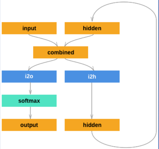
• The input is combined with the hidden state and output logits are generated using softmax along with hthe new hidden state which is used in next time step.

class RNN(nn.Module):
    def __init__(self, input_size, hidden_size, output_size):
        super(RNN, self).__init__()

        self.hidden_size = hidden_size
        self.i2h = nn.Linear(input_size + hidden_size, hidden_size)
        self.i2o = nn.Linear(input_size + hidden_size, output_size)

    def forward(self, input_tensor, hidden_tensor):
        combined = torch.cat((input_tensor, hidden_tensor), 1)

        hidden = torch.tanh(self.i2h(combined))
        output = self.i2o(combined)
        return output, hidden

    def init_hidden(self):
        return torch.zeros(1, self.hidden_size) # initializing the hidden state at the beginning of a sequence.

• self.i2h = nn.Linear(input_size + hidden_size, hidden_size)
  • It is a nn.Linear that takes concatenated input and previous hidden state to produce the new hidden state.
• self.i20 = nn.Linear(input_size + hidden_size, output_size)
  • It is a nn.Linear that takes concatenated input and previous hidden state to produce the raw output.

Training :

def train(rnn, line_tensor, category_tensor, criterion, optimizer):
    hidden = rnn.init_hidden()

    # Forward pass through each character in the name
    for i in range(line_tensor.size()[0]):
        output, hidden = rnn(line_tensor[i], hidden)

    # Compute the loss using the final output
    loss = criterion(output, category_tensor)

    # Backward pass and optimization step
    optimizer.zero_grad()
    loss.backward() # automatically performs bptt because of the way network is defined
    optimizer.step()

    return output, loss.item()

# Create RNN instance
n_hidden = 128
rnn = RNN(N_LETTERS, n_hidden, n_categories)

# Loss function and optimizer
criterion = nn.CrossEntropyLoss()
learning_rate = 0.001
optimizer = torch.optim.AdamW(rnn.parameters(), lr=learning_rate)

Detailed code can be found here

• Using nn.RNN

import torch.nn as nn
import torch.nn.functional as F

class CharRNN(nn.Module):
    def __init__(self, input_size, hidden_size, output_size):
        super(CharRNN, self).__init__()

        self.rnn = nn.RNN(input_size, hidden_size)
        self.h2o = nn.Linear(hidden_size, output_size)
        self.softmax = nn.LogSoftmax(dim=1)

    def forward(self, line_tensor):
        rnn_out, hidden = self.rnn(line_tensor)
        output = self.h2o(hidden[0])
        output = self.softmax(output)

        return output

Application of RNNs

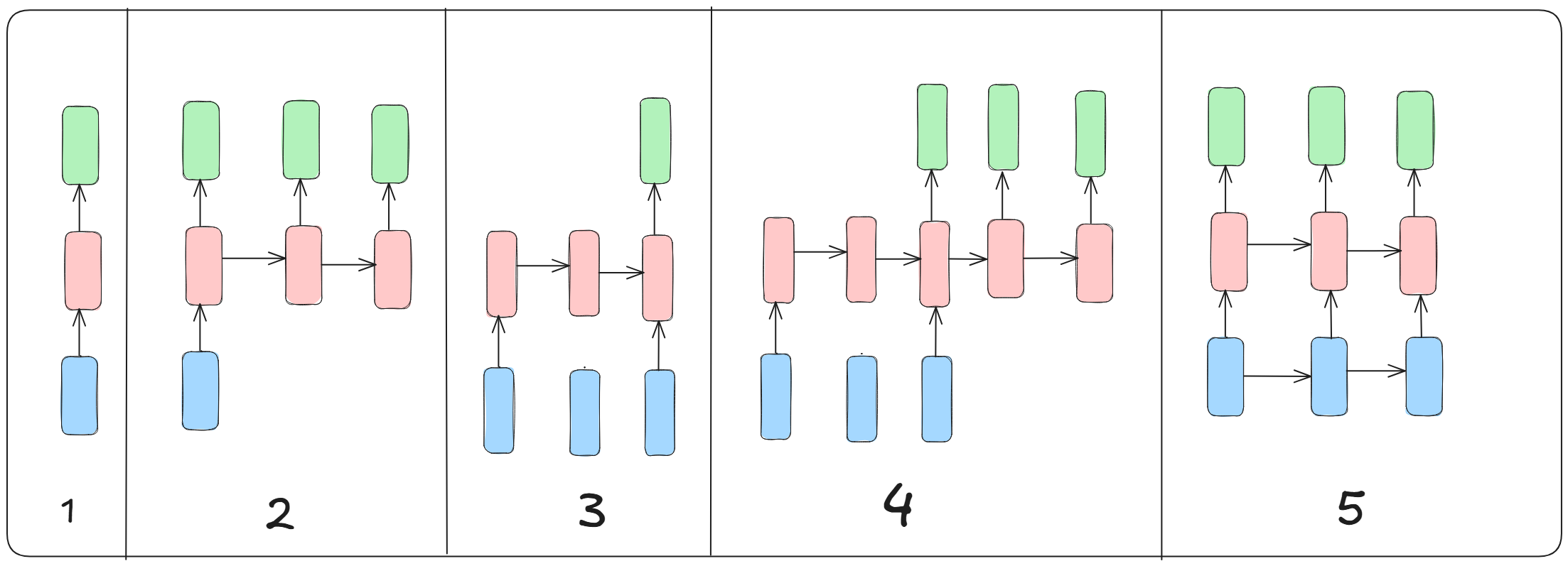
• Each arrow is function like matric multiplication.
• These arrows are connected to rectangles which represent vectors :
  • Blue : input vector
  • Red : Hidden state vector
  • Green : Output vector

1. One to One

• No RNN. It is just a normal / vanilla mode of processing, like image classification.
• From fixed sized input to fixed size output.

2. One to Many

• Gives a sequence output.
• Example : Image captioning task, where only a image is provided and the output is a sequence of words.

3. Many to One

• Input is a sequence.
• Example : Sentiment analysis, proivded a sentence check whether it is positive or negative.

4. Many to Many

• Can be used for machine translation tasks.

5. Many to Many

• Synched sequence input and output.
• Example : Video classification where each frame is labelled.

---

Bidrectional RNN (BRNN)

• 

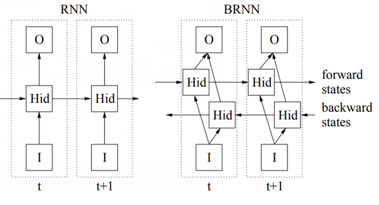
• Unlike standard RNN which only uses the past context, a BRNN can use both past and future contexts.
• It has 2 separate hidden states.
  • One processes the sequence from start.
  • Other from end.

• Outputs from both the hidden states are combined to form the final output.

• Since they consider more information, they are better at predictions.

Teacher Forcing :

• Instead of feeding its own prediction to a model as input for next time step generation, the model is fed the actual ground truth.

  At time step t, the model receives the ground truth from t-1 as input.

Advantages

• This leads to faster convergence, since ground truths are more accurate.
• Reduces the risk of the model drifting into incorrect sequences due to compunding prediction errors.

Disadvantages

• This may lead to error accumulation and poor performance at inference time.
• Exposure Bias : During inference, model won’t have access to the ground truth and must rely on its own predictions.

Scheduled Sampling / Probabilistic Teacher Forcing

• Model gradually transitions from teacher forcing to using its own predictions during training, to mitigate exposure bias.

• Implementation

import torch.nn as nn

class DecoderRNN(nn.Module):
    def __init__(self, output_dim, emb_dim, hidden_dim):
        super(DecoderRNN, self).__init__()
        self.embedding = nn.Embedding(output_dim, emb_dim)
        self.rnn = nn.GRU(emb_dim, hidden_dim)
        self.fc = nn.Linear(hidden_dim, output_dim)
    
    def forward(self, input, hidden):
        # input: (1, batch_size) => single time step
        embedded = self.embedding(input)  # (1, batch_size, emb_dim)
        output, hidden = self.rnn(embedded, hidden)  # output: (1, batch_size, hidden_dim)
        prediction = self.fc(output.squeeze(0))  # (batch_size, output_dim)
        return prediction, hidden

def train(decoder, target_seq, decoder_hidden, teacher_forcing_ratio=0.5):
    """
    decoder: the decoder model
    target_seq: tensor of shape (target_len, batch_size)
    decoder_hidden: initial hidden state from encoder or zero
    """
    target_len = target_seq.size(0)
    batch_size = target_seq.size(1)
    output_dim = decoder.fc.out_features

    outputs = torch.zeros(target_len, batch_size, output_dim)

    decoder_input = target_seq[0, :]  # Usually the <sos> token

    for t in range(1, target_len):
        output, decoder_hidden = decoder(decoder_input.unsqueeze(0), decoder_hidden)
        outputs[t] = output

        teacher_force = torch.rand(1).item() < teacher_forcing_ratio
        top1 = output.argmax(1)  # Get predicted token

        decoder_input = target_seq[t] if teacher_force else top1

    return outputs

• teacher_forcing_ratio controls the probability of using the ground truth vs. the model’s prediction.
• teacher_forcing_ratio=1.0, it’s full teacher forcing. When 0.0, the model always uses its own predictions.