2. NLP: Long Short Term Memory [LSTM] & Gated Recurrent Unit [GRU]
LSTM
-
LSTMs were developed to handle the drawbacks of RNNs, i.e., their inability to handle long term dependencies.
- LSTM are just a special type of RNN which can handle long term dependencies.
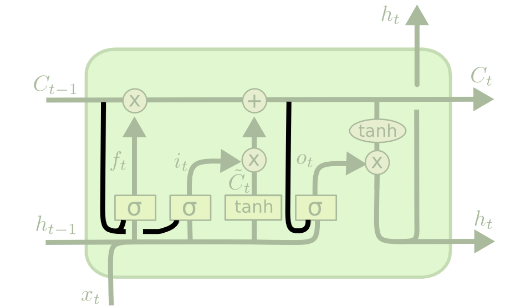
- The repeating module has a different structure as compared to a RNN (as shown in the below figure).
- red circle : pointwise operation (eg. vector addition)
- yellow rectangle : neural network layer
-
A simple RNN cell has one main neural layer : \(h_t = tanh(W_{xh}x_t + W_{hh}h_{t-1} + b)\)
-
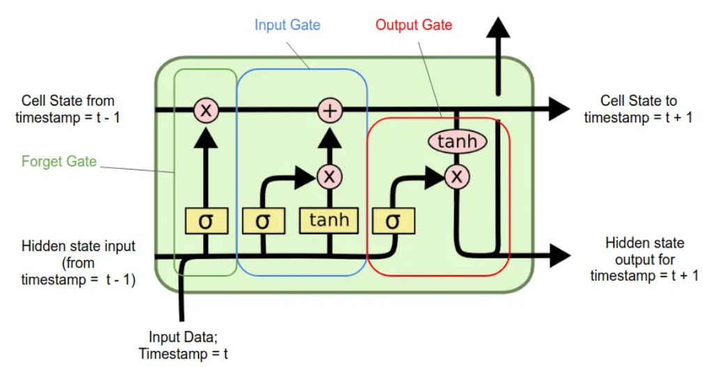
LSTM cell consists of 3 gates.
Cell State :
- It is a vector that acts as the long-term memory of the network.
- It carries important information across many time steps in a sequence.
- It is updated / modified only through gates.
Gates of LSTM
1. Forget Gate [ $ f_t $ ]
- Helps to decide what information is to be thrown away from the cell state.
- \[f_t = \sigma (W_f \cdot [h_{t-1}, x_t] + b_f)\]
2. Input Gate [ $ i_t $ ]
- Decides what new information to be stored in the cell state.
- There are 2 parts in it :
-
Input gate layer :
- A sigmoid / input gate layer decides which value will be added.
- $ i_t = \sigma (W_i \cdot [h_{t-1}, x_t] + b_i) $
-
New Memory / Candidate Layer :
- Proposes new candidate values vector to be added to the cell state using a
tanhlayer. - $ \tilde C_t = tanh(W_C \cdot [h_{t-1}, x_t] + b_C) $
- Proposes new candidate values vector to be added to the cell state using a
- These 2 will be combined to get the new cell state update.
-
3. Update the cell state [ $ C_t $]
- Updating the cell state from old $ C_{t-1} $ to new $ C_t $.
- $ C_t = f_t \circ C_{t-1} + i_j \circ \tilde C_t $
- Multiplying old state by $ f_t $ denotes the forgetting the info which was decided to be forgotten earlier.
4. Ouput Gate [ $ o_t $]
- Decide which part of the cell state is going to be the output.
- Done in 2 parts :
-
Deciding the parts going to the output
- Using a sigmoid layer
- $ o_t = \sigma (W_o [h_{t-1}, x_t] + b_o) $
-
Get the output
- Use a tanh layer for values to be in range [-1, 1].
- $ h_t = o_t \circ tanh(C_t) $
-
How LSTM solve the Vanishing Grdient Problem
-
The Cell State is the key of the LSTM.
-
Additive updates instead of multiplicative
- avoids the repeated multiplicative squashing that causes vanishing gradients.
- $ C_t = f_t \circ C_{t-1} + i_j \circ \tilde C_t $
-
Control Flow of gradients using Forget Gate
- If $f_t$ = 1 and $i_t$ = 0 then : $C_t = C_{t-1}
- Thus, the gradient can flow inchanged across many time steps.
- It provides a highway for gradients to flow.
Variations of LSTM (using peepholes)
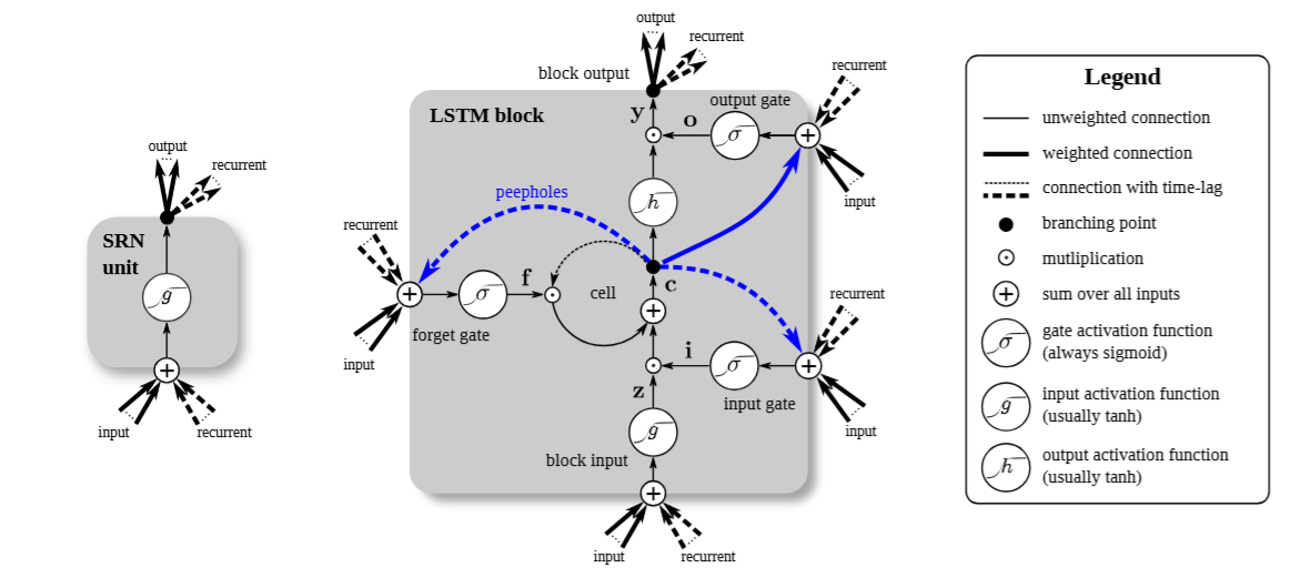
- All the gates get a direct connection to the previous cell state.
- Since the cell state $C_{t-1}$ contains richer memory than the hidden state $h_{t-1}$ , allows for more informed decision making.
Updated gate eqautions
- $ f_t = \sigma (W_f \cdot [C_{t-1}, h_{t-1}, x_t] + b_f) $
- $ i_t = \sigma (W_i \cdot [C_{t-1}, h_{t-1}, x_t] + b_i) $
- $ o_t = \sigma (W_o [C_{t-1}, h_{t-1}, x_t] + b_o) $
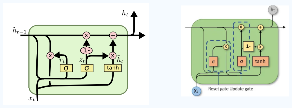
GRU
- It is a simplified variation of LSTM.
- It has fewer parameters and simpler architecture.
-
GRU removes the cell state and merges everything into a single hidden state.
- Combines Input gate and Forget gate into a single Update Gate $z_t$
- It decides how much of the past to keep vs. how much new info to add.
-
Removed the output gate, thus directly outputs the hidden state.
- Added a new Reset Gate $r_t$ to control how much past info to forget when computing the new candidate $\tilde h_t$
- $z_t = \sigma (W_z \cdot [h_{t-1}, x_t])$
- $r_t = \sigma (W_r \cdot [h_{t-1}, x_t])$
- $\tilde h_t = tanh(W \circ [r_t * h_{t-1}, x_t])$
- $h_t = (1 - z_t) * h_{t-1} + z_t * \tilde h_t$
- GRUs are faster to compute and has fewer parameters.
Implementation of LSTM in a sentiment analysis task can be found here