9. NLP: Optimizing Attention
Need for Optimizing
The original transformer’s (Vaswani et al., 2017) attention mechanism (scaled dot-product attention) has time complexity of $O(n^2 \cdot d)$, where $n$ = sequence length and $d$ = dimensionality of the embedding.
- Explanation of time complexity :
- $QK^T$ is matrix multiplication of shape $ (n \times d) \cdot (d \times n) $ which will cost $O(n^2 \cdot d)$.
- Softmax will be applied over each of the $ n \times n $ scores of the attention scores, it will cost $O(n^2)$.
- MatMul of attention matrix with $V$ will also be $O(n^2 \cdot d)$.
- Thus the overall complexity will stay $O(n^2 \cdot d)$.
-
To address this quadratic scaling of Transformer models, various new techinques have been developed.
-
Methods discussed in this post are :
- KV- Caching
- Sliding Window Attention (SWA)
- Multi-Query Attention (MQA) & Grouped-Query Attention (GQA)
Key-Value Caching : Efficient Inference
KV-Caching is used in the decoder’s self attention. It speeds up the autoregresive generation of text. To understand KV-Cache, it is important to revisit how the (causal) self attention works.
Self Attention Mechanism
Detailed explanantion of attention and transformer can be found here.
- The self attention layer of the transformer computes 3 vectors called Query, Key and Values vectors for each token in the input sequence.
- Q represents what information is needed from other words.
- K represents what each token offers in terms of information.
-
V represents the actual content/information from that token that will be retrieved if it’s deemed relevant..
- To figure out how much attention to pay to each token in the input sequence, the model will compare the query of the current token with the Keys of all other words.
- This comparision will gives attention scores.
- These scores are used to weight the values of the other words.
-
The weighted sum of values become the context for the current word, helping the model understand its meaning in relation to the entire sequence.
- This can be described mathematically as :
- It determines how much attention token $i$ should pay to token $j$.
Token-by-Token Generation (Non KV-caching)
- The generative transformer models / decoder only models append the token generated at time $t_i$ to the input at time $t_{i+1}$.
- Thus, each time the model generates a new token it will :
- Feed the entire sequence generated so far into the model.
- Recompute all the self-attention activations for all the tokens in the sequence.
- Predict the next token based on the final hidden state of the last token.
"Generate t1" -> compute attention score for  t1
"Generate t2" -> compute attention score for  t1, t2
"Generate t3" -> compute attention score for  t1, t2, t3
- Thus, for generating token t3, the model recomputes the attention scores from scratch for t1 and t2.
- It is redundant to recompute the scoresa again for earlier tokens.
Transformer Decoding with KV-Caching
KV-caching solves this redundancy by storing / caching the intermediate outputs, i.e. the keys and values vectors, from self attention layers for previous tokens.
- Thus, for each new token the model will :
- Process only the new token.
- Reuse the previously cached key-value pairs from earlier tokens.
- Append new K/V vectors for the cuurent token into the cache.
- Computes attention only between the new token and all previous tokens via the cached keys/values.
"Generate t1" -> compute & store K1, V1
"Generate t2" -> resuse K1,V1 + compute & store K2, V2
"Generate t3" -> resuse K1,V1 & K2,V2 + compute & store K3, V3
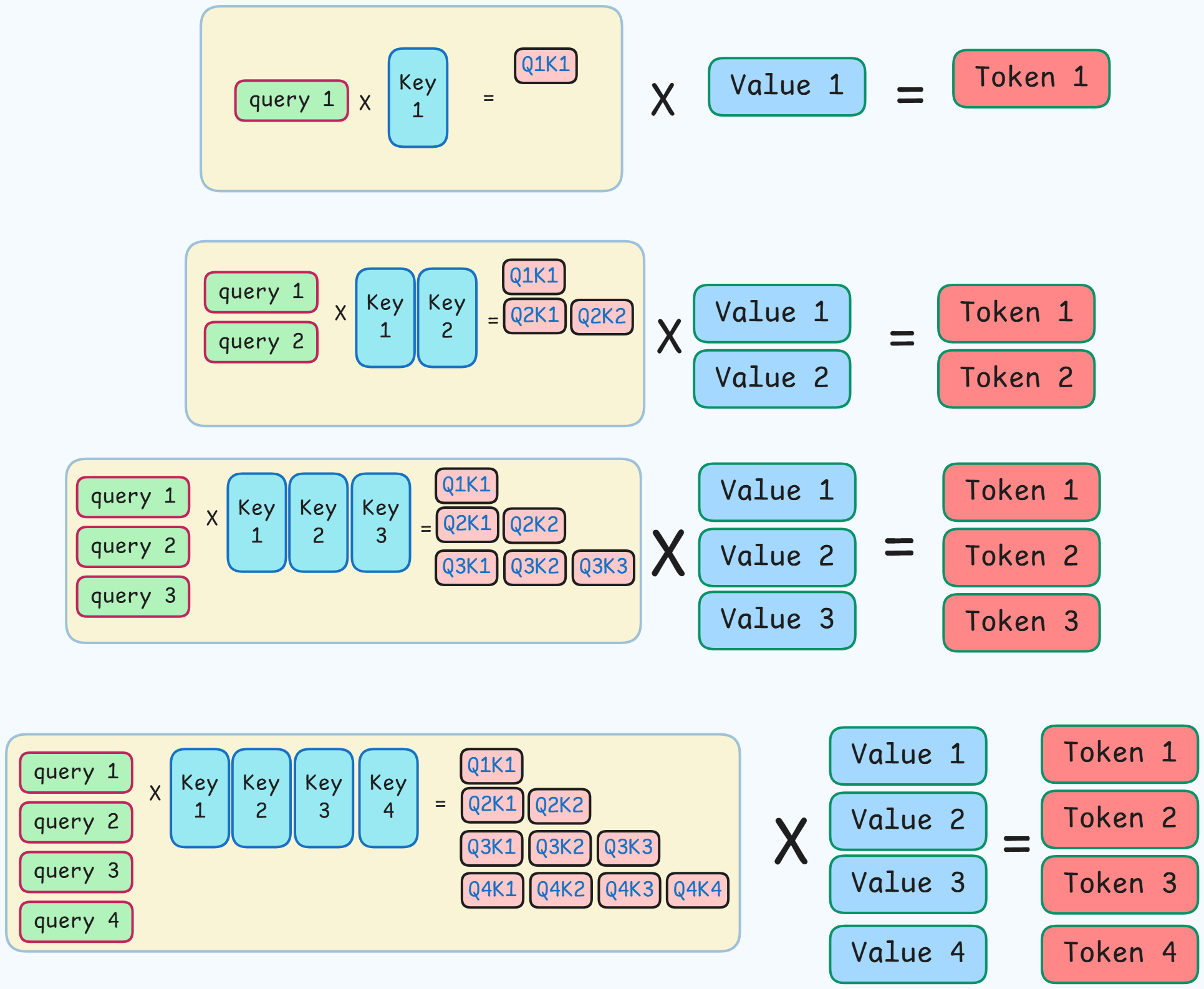
- Yellow box : scaling and applying softmax
- Red boxes : represent $QK^T$.
- Blue boxes (value & key) : represent computed vectors.
- This image shows how token generation works when KV-Caching is not being used.
-
The same Key and Value vectors are being recomputed for every token.
- To prevent this recomputation of K and V, the K and V vectors will be stored and reused for the next token genration.
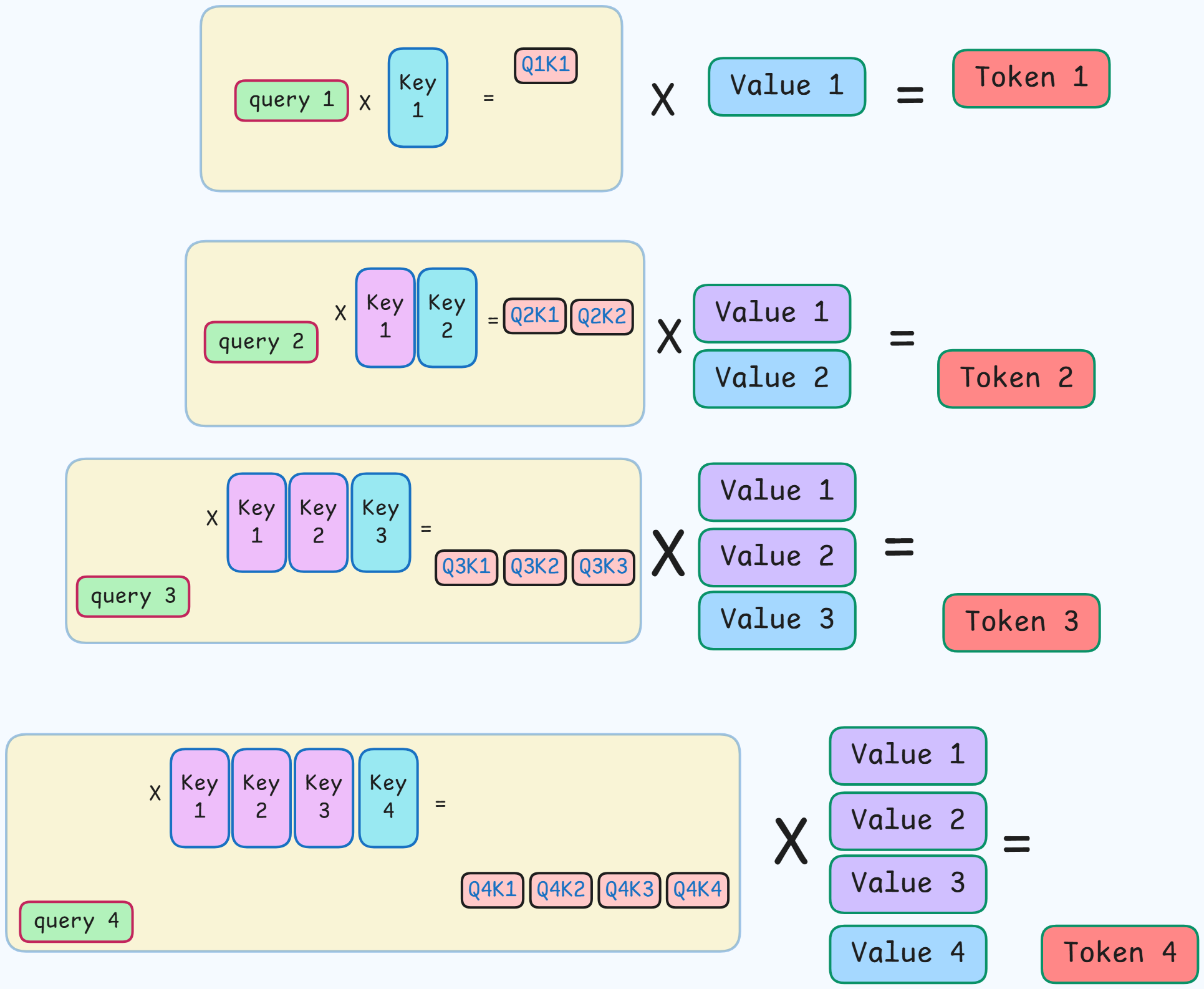
- Pink / Violet boxes : Retrived from cache
- Since the K and V vectors are already stored, there is no need to re-calculate the attention scores again.
- Thus, only the query vector of the last generated token is multiplied with the key vectors.
Thus, by storing the intermediate key (K) and value (V) vectors for all preceding tokens, the model only needs to compute the query (Q) for the current token and attend to the cached keys and values, dramatically reducing redundant computations.
Time Complexity analysis after KV-Caching
- At time step $t$, only the query $Q_t$ for the newly generated token is computed from the embedding : cost = $O(d)$.
- No recomputation for K and V from $t = 1 \, to \, t-1$, as they are already cached.
- Attention score computation will now be multiplying a single query vector $(1 \times d)$ with the cached keys $(d \times t)$ costing $O(t \cdot d)$.
- Applying softmax over $t$ scores will cost $O(t \cdot d)$ which is negligible for large $d$.
-
Multiplying the resulting $(1 \times t)$ attention weights with cached values $(t \times d)$ costs $O(t \cdot d)$.
-
Hence, total cost per time step = $O(t \cdot d)$.
- Over $n$ decoding steps / the sequence length the cost will become :
Thus, KV-Caching results in a linear time complexity instead of the previous quadratic.
Drawbacks
- Memory usgae increases with sequence length.
- Less efficient for small sequence length and high batch inference.
- With large batches, the GPU is already doing big matrix multiplies in parallel, so the extra computation from recomputing keys/values is relatively cheap, while the memory cost of KV caching grows linearly with batch size, making it a bad trade-off.
Sliding Window Attention (SWA)
- In Self-Attention, instead of every token attending to every other token, sparcity can be introduced into the attention matrix.
-
Instead of the global receptive field of self attention, the tokens attend to all other tokens in a small local recptive field.
-
The major assumption behind this approach is that, much of the semantic and syntactic information required to understand a given token is contained within its immediate vicinity.
- The full dense attention matrix of shape $N \times N$ is replaced by sparse, banded matrix.
Banded Matrix : Non-zero values are present around only the diagonal.
- Diagonal represents a token attending to itself.
- Thus, positions nearby the diagonal represent nearby tokens in the sequence.
- Each token is restricted to attend to fixed size window of w tokens around it.
-
For causal language modelling, a token position $t$ will attend to itself and preceding $w-1$ tokens around it.
- For each token $t$, attention is computed only over tokens in :
Analogy to CNNs
- A single convolutional layer in a CNN has a small, local receptive field but by stacking multiple convolutional layers, the receptive field grows larger.
-
A neuron in a higher layer can integrate information from a much wider area of the input image than a single kernel would suggest.
- A similar idea is used in SWA.
- Stacking of SWA means that multiple transformer blocks are stacked vertically each haing a SWA layer.
- Output of layer $l$ becomes the input of layer $l+1$.
- When Layer 2 runs SWA again, each token can attend to a new local window — but those tokens already contain information from their own windows in Layer 1.
Input → SWA Layer 1 → SWA Layer 2 → SWA Layer 3 → …
    A  B  C  D  E  F  G  H
A [ X  X  .  .  .  .  .  . ]
B [ X  X  X  .  .  .  .  . ]
C [ .  X  X  X  .  .  .  . ]
D [ .  .  X  X  X  .  .  . ]
E [ .  .  .  X  X  X  .  . ]
F [ .  .  .  .  X  X  X  . ]
G [ .  .  .  .  .  X  X  X ]
H [ .  .  .  .  .  .  X  X ]
Xmeans attended token and.means no attention.-
$N = 8 \quad \text{and} \quad w = 3$
-
To see how tokens indirectly influence D after each block.
- In layer 1 :
- D is directly attended by C, D, E.
- In layer 2 :
- C has information of B from layer 1.
- E has information of F from layer 1.
- Hence, D is attended by B, C, D, E, F.
- In layer 3 :
- B has information of A from layer 2.
- F has information of G from layer 2.
- Hence, D is attended by A, B, C, D, E, F, G.
- In layer 4 :
- G has information of H from layer 3.
- Hence, D is attended by A, B, C, D, E, F, G, H.
Thus, over multiple layers, SWA will get information from all tokens in the sequence, but computation in each step will be a lot less than in vanilla self attention.
    Layer_1                 Layer_2                 Layer_3
[ X X . . . . . . ]     [ X X X . . . . . ]     [ X X X X . . . . ]
[ X X X . . . . . ]     [ X X X X . . . . ]     [ X X X X X . . . ]
[ . X X X . . . . ]     [ X X X X X . . . ]     [ X X X X X X . . ]
[ . . X X X . . . ]     [ . X X X X X . . ]     [ X X X X X X X . ]
[ . . . X X X . . ]     [ . . X X X X X . ]     [ . X X X X X X X ]
[ . . . . X X X . ]     [ . . . X X X X X ]     [ . . X X X X X X ]
[ . . . . . X X X ]     [ . . . . X X X X ]     [ . . . X X X X X ]
[ . . . . . . X X ]     [ . . . . . X X X ]     [ . . . . X X X X ]
SWA reduces memory and time complexity from :
- Memory : $ O(N^2) \rightarrow O(N \cdot w) $
- Time : $ O(N^2 \cdot d) \rightarrow O(N \cdot w \cdot d) $
- Thus, SWA is effectively linear with respect to the sequence length.
Mathematical Formulation
For Standard Attention
- Output of the entire sequence :
- For a single query vector $q_t$ ($t^{th}$ row of Q), computation can be expressed as :
For Sliding Window Attention
-
SWA modifies the formulation by restricting $i$ and $j$ in the summations to a local window.
-
For a window size $w$ and a given query token $t$, attention is constrained to the set of tokens :
- Thus, output becomes :
Practical Implementation of SWA
Longformer : The Long-Document Transformer
-
It combines local window attention along with global task-specific attenion.
-
Local Attention : Majority of tokens use SWA, enabling linear scaling and only attending to their local neighbours.
-
Global Attention : A few tokens are pre-selected and are designated as global.
- They can attend to every other token in the entire sequence.
- Every other token in the sequence can attend to them.
Hence, this deign can be thought of as an information highway.
- Global tokens act as hubs as they gather info from all local contexts and broadcast important info across the document.
- If only local attention is used then if we want
token 10to attend / affecttoken 500, then information would have to hop through 100s of intermediated tokens. - Global attention bridges these long ditances by drastically reducing the hops :
token 10$\to$GlobalToken$\to$token 500.
Global Tokens
-
It is task dependent.
- Text Classification
[CLS](classification) token at the start of the sequence.- As it needs to summarize the whole text into a single representation for classification.
- Question Answering (QA)
- All question tokens become the global token.
- All passage tokens become the local tokens.
- Question tokens must access the entire passage to find relevant evidence, and the passage must access the question directly to know what to look for.
*: full connectionX: local connection
    G1  G2  L3  L4  L5 ...
G1   *   *   *   *   *  ...
G2   *   *   *   *   *  ...
L3   *   *   X   X   X  ...
L4   *   *   X   X   X  ...
...
- First two rows = global tokens $to$ every entry is active.
- First two columns = global tokens $to$ every row has them visible.
Time Complexity : $ O(n \cdot w + n \cdot g) $
- $n$ : sequence length
- $g$ : number of global tokens
- $w$ : window size
- $g$ and $w$ are relatively smaller than $n$, hence time complexity is linear in $n$.
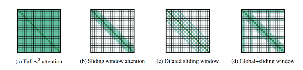
Dilated Sliding Window
- Gaps were introduced in the attention window.
- Instead of a token attending to positions $t-2$, $t-1$, $t$, it will attend to tokens at position $t-4$, $t-2$, $t$ if the dilation factor is 2.
BigBird : Formalizing Sparse Attention
- The BigBird model is combination of 3 building blocks.
- Sliding Window / local attention (identical to core SWA)
- Global Tokens (Similar to Longformer)
- Random Attention
Random Attention
- Each token will attend to small, fixed number of randomly selected tokens.
- This ensures shortcuts between far-apart tokens.
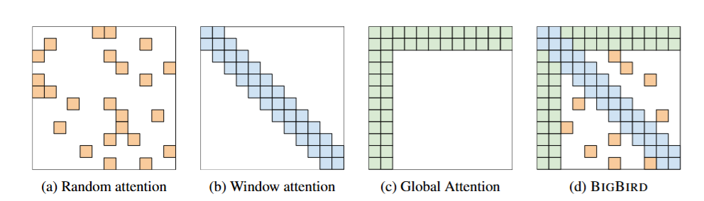
- Random attention with $r$ = 2 (each token picks 3 random other tokens).
- SWA with $w$ = 3.
- Global attention with $g$ = 2.
- Combined BigBird model.
The authors of BigBird paper also proved that sparsed attention is a universal approximator of sequence function and it is Turing complete just like the full quadratic attention model.
Universal Approximator Of Sequence Function
- It means that given sufficient width and depth, a full attention transformer can approximate any continuous sequence-to-sequence function to an arbitrary degree of accuracy.
Sequence-To-Sequence Function : A function whose input is a finite sequence of vectors (tokens, embeddings, symbols, etc.), and whose output is another finite sequence—often (but not necessarily) of the same length.
Turing Completeness
- A system is called Turing complete if it can perform any computation that a Turing machine could, given enough time and memory.
- A Turing Machine consists of :
- Tape : an infinite strip of cells
- Head : it can reas and write symbols on the tape
- Set of States : it dictates the head’s direction / action based on the current state and the symbol being read.
- Tape :
- The input and output sequence of tokens can be used to represent the history of the Turing machine’s tape.
- Each token can encode the symbol at a particular position on the tape at a specific time step.
- Head :
- Attention mechanism can be configured to simulate the movement of the Turing machine’s head.
- By manipulating the query, key, and value matrices, the attention scores can be made to focus on the token representing the current position of the head on the tape.
- Use hardmax instead of softmax here, as it allows the model to attend to a single, specific token, mimicking the focused action of the read/write head.
- State Transitions :
- The FFNs within the Transformer can be programmed to implement the transition function of the Turing machine.
- Based on the current state (which can also be encoded in the token representations) and the symbol read from the “tape” (the attended-to token), the feed-forward network can compute the next state, the symbol to be written, and the direction to move the head.
- The BigBird’s author argued that for a sparse attention model to be a universal approximator, information must be able to flow efficiently between any two nodes (tokens) in the sequence within a small number of layers.
- Using the combination of 3 types of attentions, the full attention matrix can be approximated.
- Because the underlying graph structure allows information to propagate fully and efficiently, the model retains the expressive power of a standard Transformer and is thus a universal approximator of sequence functions.
- Because the global tokens can access any token in the sequence in a single step, the model can simulate the arbitrary movement of a Turing machine’s head.
- Thus the BigBird architecture is turing complete.
- Time Complexity : $ O(n (w + r + g)) $
- $r$ : random links
- $g$ : number of global tokens
- $w$ : window size
- Thus, it effectively linear in $n$.
Drawbacks of SWA : Attention Sink
It is a phenomenon in auto-regressive language models where the model allocates a disproportionally high amount of attention to a few (semmantically unimportant) tokens.
- The attention mechanism calculates a score for how much a query token should attend to each key token.
- These scores are then normalized using a softmax function, ensuring them some up to 1.
If a query token doesn’t have any symantic connection to any of the key tokens in the context, softmax will force the attention scoret to be distributed among all available key tokens.
- The initial tokens of the sequence will always be visible to all subsequent tokens of the sequence in an auto-regressive model.
-
Thus, the model learns to funnel the unneeded attention to these tokens.
- In Longformer & BigBird :
- The global tokens or the initial token act as the attention sink.
Attention sink problem is more prominent in sparse attention models as less number of global tokens are used thus acting as the only path for long-range interaction and thus a bottleneck.
- This can cause information compression loss and overfitting to the sink tokens.
High variance introduced by the softmax operation makes the global token more bottlenecked and unstable
- Variance : how much the attention weights for different tokens fluctuate across different queries and across training steps.
- High variance : very peaky attention (one or two tokens get huge weights, others get almost zero).
- Low variance : weights are more evenly spread out.
- Softmax exaggerates small score differences, amplifies variance.
- Let :
- Local 1: score = 1.0
- Local 2: score = 0.9
- Local 3: score = 0.8
- Sink token: score = 1.2
- Summing up the exponentiated scores will give 10.73
- Thus sink weight = 3.32 / 10.73 = 0.31 ($e^{1.2} = 3.32$)
- If sink score increases by just 0.2 to 1.4 :
- sink weight = 4.05 / 11.46 = 0.35
- Thus, a tiny change in score (+0.2) gave the sink a 13% relative boost in weight.
- If this keeps happening across many queries, it will resulr in unstable attention maps.
SWAT: Sliding Window Attention Training
It tackles the attention sink problem by :
1. Use Sigmoid instead of Softmax
- Softmax is like “winner-takes-most” voting : tiny score boosts cause huge weight shifts (high variance).
-
Sigmoid is like “independent scoring” : small score boosts cause small weight shifts (low variance).
- $\sigma(\cdot)$ is element-wise sigmoid, thus it will not force tokens to compete for a fixed budget attention probabilities.
- This leads to more tokens getting higher scores simultaneously.
- This creates denser attention weights, encouraging the model to learn to compress and retain information from a wider range of tokens within its window.
2. Use ALiBi : Attention with Linear Biases
-
Instead of adding positional embeddings to token vectors, ALiBi modifies the attention scores directly by adding a bias proportional to the distance between tokens.
-
Compute raw attention score :
- Substract a bias proportional to the distance :
- $m$ is a fixed slope.
- It injects positional awareness without requiring extra tokens or embeddings.
- It gives a strong local preference.
3. Use RoPE : Rotary Position Embeddings
- Instead of adding a number to represent position, RoPE rotates the query and key vectors in the complex plane by an amount proportional to their position index.
-
It bakes relative position awareness into the dot product itself.
- For each position $p$ and each embedding dimension pair $(x_{2i}, x_{2i + 1})$ , apply a rotation :
- Spilt the q/k vector into pairs of dimensions : $(x_0, x_1), (x_2, x_3), \cdot$
- For each pair index $i$ : $ \theta_i = 10000^{- \frac{2i}{d_k}} $
- For position $p$ :
- $ \Theta_{p,i} = p \cdot \theta_i $
- Rotate queries and keys before taking the dot product : $ score_{mn} = (R_mq)^T (R_nk) $
- $m$ : position of the query
- $n$ : position of the key
Rotation matrices $R$ are orthogonal ($R^T = R^{-1}$)
- $R_a$ : the rotation matrix corresponding to a rotation by angle $a$.
- $R_a^T = R_a^{-1}$ : rotate by $-a$
- $R_a^TR_b = R_{-a}{b}$
- First rotate by $b$
- Then rotate by $-a$
- This is equivalent to rotating by $b-a$
- $R_a^TR_b = R_{b-a}$
- Hence, $ (R_mq)^T (R_nk) $ can be written as :
- $ = q^T R_m^T (R_nk) $
- $ = q^T R_{-m}/ (R_nk) $
- $ = q^T R_{n-m} k $
- The absolute positions $m$ and $n$ never appear separately anymore.
- Only the difference $n-m$ matters.
- That means the attention score is inherently relative position aware — It doesn’t matter where the tokens are, only how far apart they are.
Hence, the final sigmoid sliding-window attention can be formulated as :
\[Attention(Q,K,V)_m = \sum_{n=w-\omega +1}^m \sigma \left(\frac{(R_{d_{\Theta},m} q_m)^T (R_{d_{\Theta},n} k_n)}{\sqrt{d_k}} + s \cdot (m-n) \right) v_n\]- Where,
- $m$ : current query vector
- $n$ : key position within the window of size $\omega$
- $R_{d_{\Theta},m} q_m$ : rotation matrix from RoPE for position $m$
Hence, SWAT enables effective information compression and retention across sliding windows without complex architectural changes
With this, Sliding Window Attention part comes to an end.
Architectural Redesign : MQA and GQA
During autoregressive infernece a large amount of data must be transfered from main GPU memory to on-chip cache at every single step.
- To minimize this memory overhead, a redesign of Multi-Head Attention (MHA) is done. This issue comes due to KV-Cache.
-
At each generation step, the entire cache—containing the key and value vectors for all previous tokens, across all attention heads, and all layers—must be loaded from the GPU’s large but relatively slow High-Bandwidth Memory (HBM) into the small but fast on-chip SRAM where computations actually occur.
- These data transfers become the primary factor limiting inference speeds.
- Where :
- $N_L$ : number of decoder layers
- $B$ : batch size
- $S$ : sequence length
- $N_H$ : number of attention heads
- 2 : accounts for storing both keys and values
- $bytes\,per\,param$ : 2 for 16 bit floating point precision
Thus, cache size grows linearly with the number of attention heads.
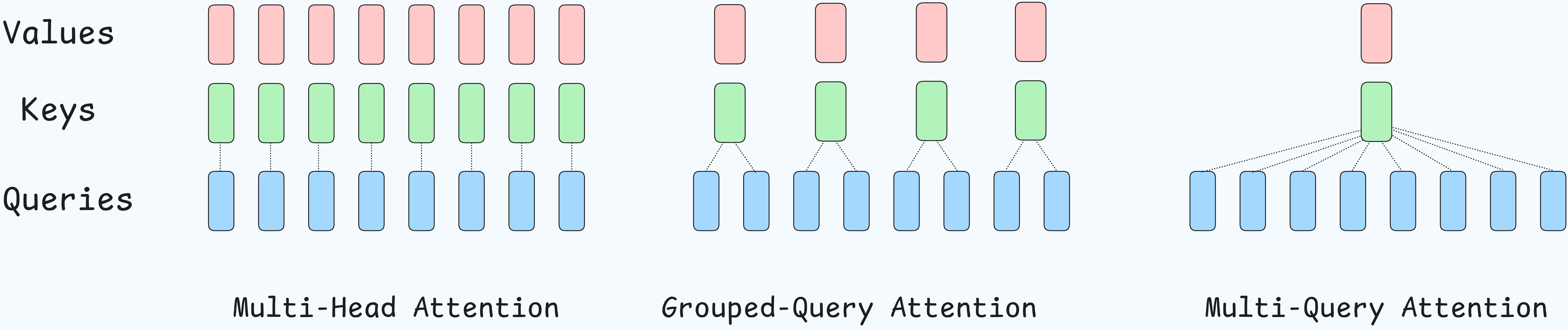
Multi-Query Attention (MQA)
-
In standard MHA, each of the query heads $N_H$ has its own corresponding key and value projection matrices, resulting in $N_H$ unique key and value heads per layer.
-
MQA changes this by modifying the arhitecture, there are still multiple query heads, but they all share a single key head and a single value head.
Effetively redued $N_H$ fator in cache size to just 1.
- Reduces size of KV-Cache and thus the amount of data loaded HBM at each time step.
Drawbacks
- The drastic reduction in parameters come at the cost of performance.
- Model loses its reoresentational capacity because the shared K/V projections must learn a single function that serves all the different query subspaces.
- This also causes training instability.
Grouped-Query Attention
- It acts as a generalization in between the extremes of MHA and MQA.
- GQA divides the total number of query, $N_H$, heads into $G$ groups.
- Each group of query heads shares a single key and value head.
- If $G$ = $N_H$, i.e. number of groups is equal to the number of query heads, then GQA is mathematically equivalent to MHA.
- Each query head has its own group.
- If $G$ = 1, then GQA is mathematically equivalent to MQA.
- All query heads are in a single group.
How MHA, MQA & GQA affect KV-Cache ?
MHA
Shapes after initial projection and transpose(1,2) :
- Queries : $ Q \in (b, H_q, s, d) $
- Keys : $ K \in (b, H_q, s, d) $
- Values : $ V \in (b, H_q, s, d) $
$H_q$ is the number of query heads which is same as number of K/V heads here.
-
Attention Scores : $ QK^T \implies (b, H_q, s, s) $
-
KV cache size : $ O(b \times s \times H_q \times d) $
Thus, every query head has its own Key-Value Head, hence maximal memeory usage.
MQA
Shapes :
- Queries : $ Q \in (b, H_q, s, d) $
- Keys : $ K \in (b, \textbf{1}, s, d) $
-
Values : $ V \in (b, \textbf{1}, s, d) $
- Attention Scores : $ QK^T \implies (b, H_q, s, s) $
Each query heads independently, but to the same single K/V head.
- KV cache size : $ O(b \times s \times \textbf{1} \times d) $
Thus, all query heads share the same K/V heads, hence minimal memory storage.
GQA
Shapes :
- Queries are reshaped into groups :
- Keys and Values are broadcasted at compute time
- Attention scores :
- KV cache size : $ O(b \times s \times H_{kv} \times d) $
Uses less memory than MHA, but still allow numerous queries for expressivity.
- For smaller models and when model quality are the primary concern, MHA is the favoured.
- MQA is inefficient in case of multiple GPU operations.
- The same, single key and value head will have to be replicated on every single GPU in the parallel tensor processing group.
- This leads to redundant computations.
- Thus, it can be optimal for single GPU system but inefficient for multi-GPU environments.
- GQA can be parallelized easily by distributing the key-value heads across the GPUs.
- If there are 8 GPUs and 8 K/V groups, then each GPU can be responsible for each group.
- Thus, it is an optimal option for multi-GPU systems as tensor parallelism is quite high.
With this the methods to increase the efficiency of standard Multi-Head Attention comes to an end. We discussed KV-Caching, Sliding-Window Attention, Multi-Query Attention & then finally Grouped-Query Attention. These methods (KV-Caching & SWA) were devloped to reduce FLOPs (Floating Point Operations) while MQA and GQA were developed to reduce to address the increasing use of memory size due to use of KV-Caching.