What is MoE?

Mixture of Experts or MoE is a type of ensemble models that combines several small expert sub-networks.
Instead of relying on a single, monolithic model to master a vast and complex problem space, the MoE approach decomposes the problem into smaller, more manageable subproblems.

In context of Transformers

The dense Feed Forward Network (FFN) layer is replaced with the MoE layer.
It consists of two main elements :
Sparse MoE Layers
- They have a certain number of experts / FFNs.
- They are sparse as only a few are active at any given time, depending on the nature of the input.
Gate Network or Router
- It determines which tokens are sent to which expert.
- The router is composed of learned parameters and is pretrained at the same time as the rest of the network.

Thus, an MoE model routes different types of data to experts that have been trained to become highly proficient in handling those specific patterns, resulting in a more capable and efficient system overall.

History of MoEs

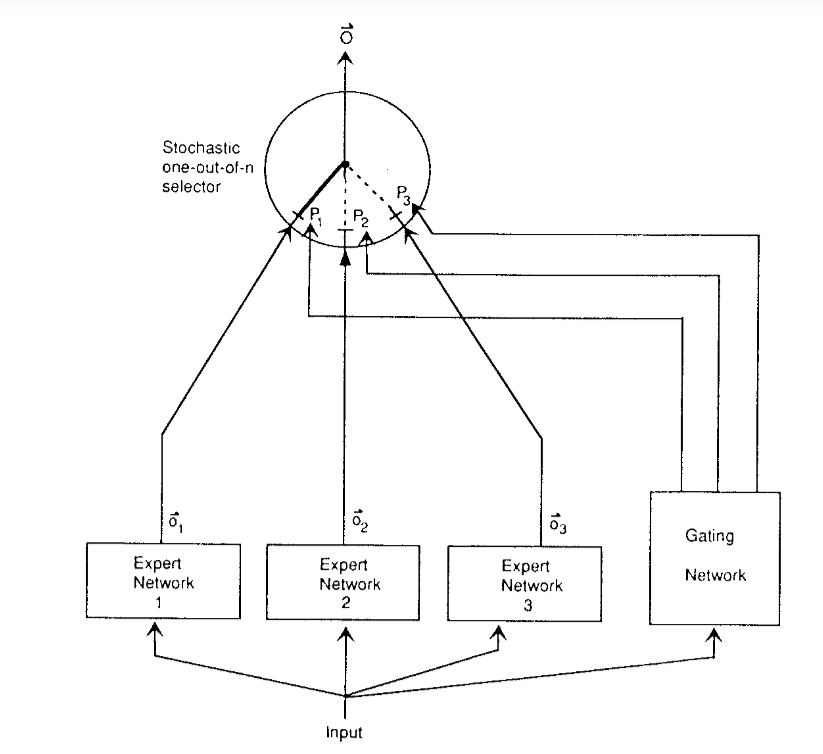
The first formal introduction of MoE was done in the paper Adaptive Mixtures of Local Experts, long before the rise of deep learning and the transformer architecture, in 1991.

It was explored as a machine learning technique for tasks like classification and regression, where multiple simple models (e.g., linear regressors or small neural networks) would specialize in different regions of the input data space.
The gating network would learn to partition this space, assigning different inputs to different experts.
The final prediction was often a weighted combination of the outputs from all experts, with the gating network providing the weights.

Diff. b/w Early work & Modern practices of MoE

Early	Modern
Each expert was a small neural network (MLPs)	Each expert is a FFN block inside a Transformer layer
Final output is weighted average of all experts, weighted by probability distribution over experts by gating network	Gating is sparse, only top-k experts are activated per token, reduced compute cost compared to activating all experts
Designed to partition the input space, each expert should specialize in different data regions.	Goal is to scale model capacity without proportional compute increase.
The gating network was trained jointly to learn this partitioning.	Additional losses are added to ensure experts don’t collapse.

Sparsely Gated MoE & Conditional Computation

The idea of MoE was scaled to LSTMs by introducing sparsity which allowed to keep fast inference even at high scale in the paper OUTRAGEOUSLY LARGE NEURAL NETWORKS:THE SPARSELY-GATED MIXTURE-OF-EXPERTS LAYER

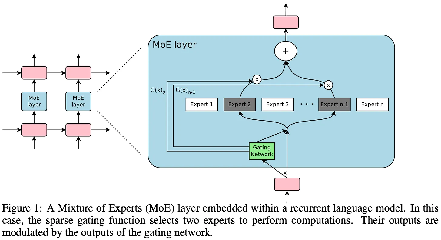
Sparsity / conditional computation means only running some parts of the whole system, unlike traditional dense model where all the parameters are used for all the inputs.

Structure of the MoE Layer

$n$ expert networks [$E_1, E_2, \cdots, E_n$].
A gating network $G$ whose output is a sparse $n$-dimensional vector.
Each expert is a FFN with identical architecture but with different parameters.
$G(x)$ : output of gating network
$E_i(x)$ : output of $i^{th}$ expert, where $x$ is the input to the MoE and $y$ is the output of MoE module.

\[y = \sum_{i=1}^n G(x)_i E_i(x)\]

The output of router is a $n$ dimensional sparse vector.
- This sparsity allows the use of only a portion of model’s parameters at any given time.
- When $G(x)_i = 0$ , then there is no need to compute $E_i(x)$.

Gating Mechanism

The simplest approach was to multiply a weight matrix with the input and apply softmax to the product.

\[G_{\sigma}(x) = softmax(x \cdot W_g)\]

Drawback : It does not guarantee that the selection of experts will be sparse.
- Thus, a modified mechanism was used which added noise and sparsity.

\[G(x) = Softmax(KeepTopK(H(x), k))\]

Where :
- \[H(x)_i = (x \cdot W_g)_i + StandardNormal() \cdot Softplus((x \cdot W_{noise})_i)\]
  - $(x \cdot W_g)_i$ : score of expert before adding noise
  - $StandardNormal()$ : a random variable drawn from a standard Gaussian distribution
  - $Softplus(z) = \log{1 + e^z}$ : smooth, always positive function.
- \[\text{KeepTopK}(v, k)_i = \begin{cases} v_i, & \text{if } v_i \text{ is in the top-}k \text{ elements of } v \\ -\infty, & \text{otherwise} \end{cases}\]
  - Router outputs after top $k$ are set to 0 (by softmax).

Noise is used as an exploration factor, so that unused experts get a chance to be picked.

Balancing the Utilization of Experts

An issue with MoE is that it converges to a state where it selects same set if experts for all inputs.

It is termed as a self-fulfilling loop because if an expert is selected more frequently, it will be trained more rapidly and will be preffered over other experts.

It is dealt by using a Load Balancing Loss.
\[Importance(X) = \sum_{x \in X} G(x)\]
- $X$ : Batch of inputs
- $G(x)$ : Gating vector for input $x$.
- It computes, foe each expert how much total gate weight it recieved from the whole batch.

If expert $i$ is choosen often then $Importance_i$ will be high.

Thus is gives a measure of imbalance.

\[L_{importance}(X) = w_{importance} \cdot CV(Importance(X))^2\]
- $CV(\cdot)$
  - Coefficient of Variation
  - $ CV(y) = \frac{\sigma(y)}{\mu(y)} $
  - It measures how spread out values are compared to their average.
  - If some experts dominate , $CV$ is high, loss grows quickly, penalizes the model for imbalance in expert usage.
- $w_{importance}$
  - hyperparameter that controls how strongly this regularization is weighted.

The MoE layer is applied convolutionally across time.

Same set of experts is shared across all time steps.

Each time step’s hidden vector is treated like an independent token going through the MoE layer.

The gating and expert selection happen for each vector independently, but the computation is batched for efficiency.

MoE in Transformers

MoE were applied successfully in encoder-decoder transformer in Switch Transformers, by converting the feed-forward layers of the model into MoE layers.

Each token is passed individually through feed-forward / MoE layer.
- Thus, each token is individually routed to its set of corresponding experts.

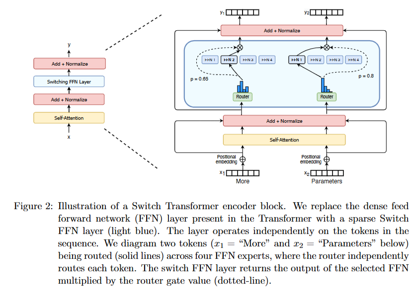
Top-1 Routing

Instead of routing to Top-$N$ experts, the token is routed to only 1 token.
This reduces computation & communication costs, while improving the model’s performance.
This is called a switch layer.
\[p_i(x) = \frac{e^{h(x)_i}}{\sum_{j=1}^N e^{h(x)_j}}\]
- Router is small linear layer with weights : $W_x$
- For an input token’s vector ($x$), router computes score :
  - $ h(x) = W_r \cdot x $
  - It is a vector of size : $N = $ number of experts.
- Then a softmax transformation is applied to convert this into a probability distribution over experts ($ p_i(x) $)
\[y = \sum_{i \in T} p_i(x) E_i(x)\]
- $T$ : top-$K$ experts
- This represents the final output of MoE layer :
  - weighted sum of the expert outputs, weighted by the gate values.
Since, only $1$ expert is to be choosen ($k = 1$) :
\[y = E_{i^*}(x)\]
- \[i^* = \arg\max_{i} p_i(x)\]
  - argument of maximum or which index $i$ makes p_i(x) largest.

Load Balancing

\[loss = \alpha \cdot N \cdot \sum_{i=1}^N f_i \cdot P_i\]
- $N$ : number of experts
- $\alpha$ : small hyperparameter
- $f_i$ : fraction of tokens that actually get dispatched to expert $i$
- $P_i$ : fraction of router probability mass that expert $i$ receives

Where :

\[f_i = \frac{1}{T} \sum_{x \in B} 1\{\arg\max p(x) = i\}\]
- $B$ : mini-batch of tokens of size $T$
- $p(x)$ : router probability for token $x$
- $\arg \max p(x)$ : the choosen expert for token $x$
- $ 1 { \cdot } $ : indicator function (1 if condition is true, else 0)
  - Here it will be true when the choosen expert is $expert_i$
- So it tells, out of the total number of tokens, how many token’s choosen expert is $expert_i$.
\[P_i = \frac{1}{T} \sum_{x \in B} p_i(x)\]
- $p_i(x)$ : probability mass assigned to expert $i$ for token $x$.
- Higer value of $P_i$ means router gives high probabilty to expert $i$.
- It measures how much the router wants to use expert $i$, even if argmax ignores it.
  - It is the average probability mass across the batch that router assigns to expert $i$.

So,

$f_i$ : gives hard usage, i.e., the actual routing of the token
$P_i$ : gives soft preference, because it takes into acount the intended preferences of the router.

Balanced Case

$f_i = 0.25 \quad \& \quad P_i = 0.23 \quad \forall \, i$

$ \sum f_i P_i = 4 * (0.25 \cdot 0.25) = 4 $
$ L_{balance} = \alpha \cdot 4 \cdot 0.25 = \alpha $

Imbalanced Case

$f_1 = 0.9 \quad \& \quad P_i = 0.9 $
For others $f_i = 0.033 \quad \& \quad P_i = 0.033$

$ \sum f_i P_i = 0.813 $
$ L_{imbalance} = \alpha \cdot 4 \cdot 0.813 = 3.25\alpha $

Thus, in imbalance case higher loss will push towards balance.

Expert Capacity

If too many tokens in a batch get routed to the same expert can lead to problems :

Training could stall because some experts are overloaded while others are idle.
That expert’s computation could blow up in memory/latency.

Thus it is necessary to control how many tokens an expert can process per batch.

Give each expert a capacity limit : the max. amount of tokens it can accept in 1 forward pass.

\[capacity = \left\lceil \frac{C_f \cdot T}{N} \right\rceil\]

Where:

$T$ : batch size
$N$ : number of experts
$C_f$ : capacity factor (hyperparameter)
$\frac{T}{N}$ : average number of tokens per expert if distribution was balanced.

If capacity is exceeded, i.e., more tokens want to go to an expert than it can hold, then :

extra tokens are dropped and are passed to the next layer by residual connections.

ST-MoE / Router $z$-loss

In the paper ST-MoE: Designing Stable and Transferable Sparse Expert Models, they introduced router $z$-loss to resolve stability issues and slightly improves model quality too.

Why Balancing loss is not enough ?

1. Logit Explosion

Router produces logits $z = (z_1, \cdots z_N)$.
- It was mentioed as $h(x)_i$ earlier under Top-1 Routing topic.
Routing probabilities come from softmax :

\[p_i = \frac{e^{z_i}}{\sum_{j=1}^N e^{z_j}}\]

Softmax is invariant to shift

Example :

\[z_i^{'} = z_i + c\] \[p_i^{'} = \frac{e^{z_i + c}}{\sum_j e^{z_j + c}} = \frac{e^c e^{z_i}}{e^c \sum_j e^{z_j}} = p_i\]

Softmax is sesitive to scaling

\[z_i^{'} = k \cdot z_i\]

If $ k \rightarrow \infty $
- Softmax becomes hard max
- If logit $z_m$ is larget among all the logits, then $e^{z_m}$ will dominate the denominator, thus :
  - $p_m^{‘} = 1$ and $ p_{i \ne m}^{‘} = 0$
- Thus, it picks the single largest logit with probability ~ 1
If $ k \rightarrow 0 $
- Softmax becomes uniform
- If $k$ is very small, then $ kz_i \approx 0 \, \forall i $
- Thus, $ e^{kz_i} \approx 1 \, \forall i $
- This leads to : $ p_i^{‘} \approx \frac{1}{n} $
- It gives equal weight to all options.

Thus,

Very large logits lead to very sharp distributions.
When one probability is near 1 and others near 0, gradients for most experts vanish.
The chosen expert’s gradient may explode because of the exponential factor.

2. Degenerate Routing

Example :

In balance loss (discussed above (switch transformer)) :
- If $N = 2$ and 2 tokens :
  - Token 1 logits : $z = (100, 0)$. Probability = (1,0).
  - Token 2 logits : $z = (0, 100)$. Probability = (0,1).
- $f_1 = f_2 = 0.5$
- $P_1 = P_2 = 0.5$
Balance loss is perfectly minimized but, each routing was extremely confident.
There’s no uncertainty or flexibility left.
If token distributions shift, the model might struggle (poor generalization).

Thus, using just the balance loss might lead to brittle and unstable training.

To fix this router $z$-loss was introduced.

Router $z$-loss

\[L_z(z) = \alpha \cdot \left(\log{\sum_{j=1}^N e^{z_j}} \right)^2\]

Where :

$\alpha$ : small coefficient (0.001)
$\log{\sum_{j=1}^N = e^{z_j}}$ : log-sum-exp (LSE)
- Smooth maximum of the logits.
Log-sum-exp grows latge if any $z_j$ is very large.
Squarring it penalizes extreme logit magnitudes.

Thus it keeps the router logits in a reasonable range, preventing them from overconfident (peaky) softmax distribution and by also prevents exploding gradients from very latge exponents.

$\therefore$

\[L = L_{task} + L_{balance} + L_{z}\]

$L_{task}$ : eg. cross-entropy loss

Mixtral 8x7B

It consists of 8 distinct FFN within each MoE layer.
It is a Top-2 model, as the router network selects the top 2 most suitable experts to process the information.
Total number of parameters are almost 47 billion but it only uses around 13 billion active parameters for any given token during inference.

Pros & Cons of MoE

Advantages

Computation Efficiency

MoE models have a massive number of parameters but don’t use all of them for a given input.
This leads to much faster inference compared to a dense model of the same size.

Scalability

MoE offers a clear path to scale models to trillions of parameters without a proportional increase in computational cost.

Disadvantages

Training Complexity

Prone to instability
Load balancing adds more complexity
Neads huge datasets to use

High VRAM Usage

All the parameters have to loaded (47B) into the memory even if only some (13B) parameters are used at a time.

10. NLP: Mixture of Experts (MOE)