Architecture

The Convolutional Neural Network consists of multiple types of layers.
1. Convolutional Layer
2. Pooling Layer
3. Fully Connected Layer

Convolutional Layer

The trainable parameters of this layer are called filters or kernels.
This layer applies the filters to the input image, extracting essential features such as edges, textures, and patterns.
Mathematical formula of convolution :
- \[O(x,y) = \sum_{c=0}^{C-1} \sum_{i = 0}^{K-1} \sum_{j = 0}^{K-1} W_c(i,j) \cdot I_c(x+i, y+j)\]
  - O(x,y) is the output feature map at position (x,y).
  - I(x+i, y+j) is the input feature map or image pixel at channel c, and spatial location (x+i, y+j).
  - W_c(x,y) is the filter of size (K,K), for input channel c.
  - K is the size of the kernel.
  - c is the number of input channels.
  - The 3 summations iterate over :
    1. c = 0 to C-1 (input channels).
    2. i = 0 to K-1 (kernel height).
    3. j = 0 to K-1 (kernel width).
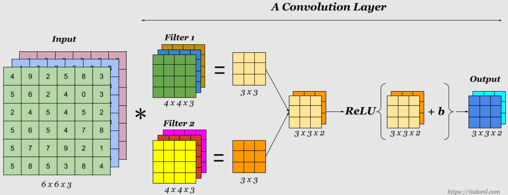
Each layer has C slices.
- C : the number of input channels.
Element wise product is performed between each filter slice and its corresponding input channel.
The results of these multiplications (for all slices) are summed together to form a single value at that spatial location.
Store the final sum in the output feature map at the corresponding position.
Slide the filter over the entire input to repeat this process for all spatial positions.
Each filter produces one output channel, so if we apply M filters, we obtain M output channels.

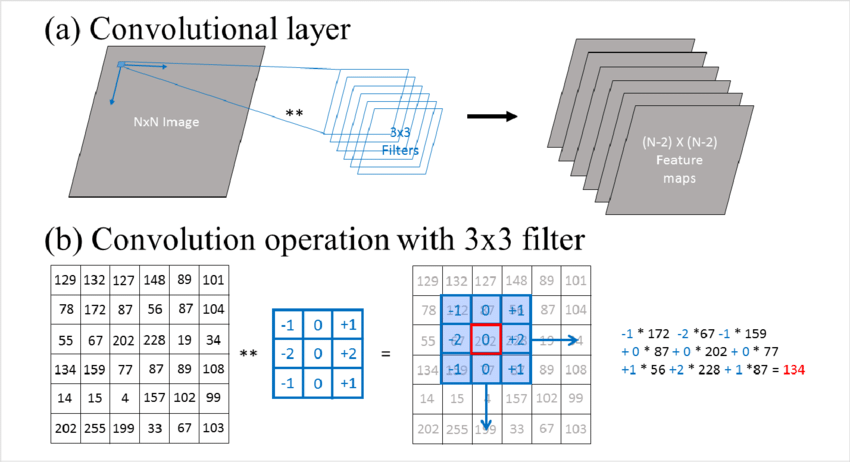
This convolution process is also called cross-correlation in CNNs.

Paramenters of Convolutional layer

conv2d of Pytorch

1. `kernel_size`

The size of the kernel used (height x width)
Larger kernel sizes capture more context but reduce spatial resolution.
It can be entered in 2 ways
- 3 : 3 x 3 kernel
- (5, 5) : 5 x 5 kernel

2. `stride`

The step size by which the filter moves across the input.
- stride=1 : the filter moves one pixel at a time (default setting).
- stride=2 : the filter moves two pixels at a time (reducing output size).
Higher stride reduces spatial dimensions (downsampling).

3. `padding`

Extra pixels added around the input before applying convolution.
- padding=0 : No extra pixels (default).
- padding=1 : Adds 1 pixel border around the input.
Preserves spatial size
Prevents information loss at the edges.
It can also be string
- padding='valid' is the same as no padding
- padding='same' pads the input, so the output has the shape as the input.

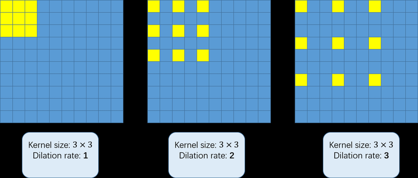
4. `dilation`

Expands the receptive field by spacing out filter elements.
- dilation=1 : Normal convolution.
- dilation=2 : Inserts 1 zero between filter elements (increases receptive field).
- dilation=3 : Inserts 2 zeros between elements.
Larger receptive field without increasing filter size.

A 3×3 filter with dilation=2 behaves like a 5×5 filter but with fewer parameters.

5 `in_channels` & `out_channels`

in_channels : Number of channels in the input image
out_channels : Number of channels produced by the convolution`

Formula for output size : \(O = \frac{W-F+2P}{S}\)

O : Output size

It can represent the height or width of the output.

W : Input size

It can represent the height or width of the input.

F : Filter / Kernel size

S : Stride

P : Padding size

Depth of the output = Number of kernels.

The convolutional layer is followed by an activation function.

Because the convolution operation is linear (It is basically weighted sum + bias (optional)).

Without an activation function, stacking multiple convolutional layers would still result in a linear transformation, limiting the network’s ability to learn complex features.

Thus, non-linearity needs to be introduced for the model to capture more abstract and high-level features.

Some terms regarding CNNs

The same set of filters (kernels) is applied across the entire input feature map (this is called parameter sharing).
This reduces the number of parameters and helps in learning spatially invariant features (e.g., detecting an edge anywhere in an image).

2. Receptive Field

The portion of the input image that a specific neuron in a convolutional layer “looks at” or is connected to, influencing its output.

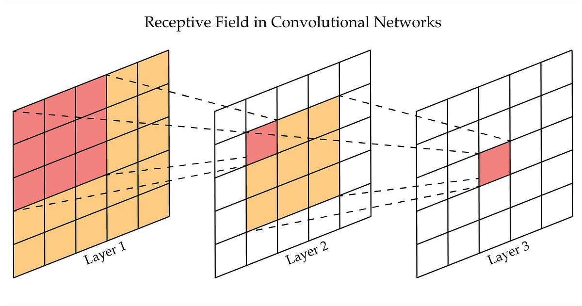
3. Local Connectivity

Unlike fully connected networks, each neuron in a CNN is only connected to a small local region (receptive field) of the input.
This reduces the number of connections and makes CNNs efficient for handling high-dimensional data like images.
Example: In a 32×32 image, a 3×3 filter connects to only 9 pixels at a time, instead of all 1024 pixels.

This leads to CNNs to having a smaller number of parameters.

Pooling Layers

Pooling layers are used to reduce the spatial dimensions of feature maps while preserving important features.
This helps in reducing computational cost and making the network more robust to small translations of the input.
Downsampling is happening.

Types of Pooling

Max Pooling
Average Pooling

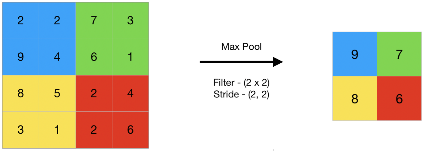
Max Pooling

Mostly used.
Selects the maximum value from each region of the feature map.
Helps retain the most important features (e.g., edges, textures).
Makes CNNs translation invariant (small shifts in input don’t affect results).
In PyTorch : MaxPool2d
- Same parameters as conv2d discussed above.

Average Pooling

Computes the average of all values in a pooling window.
Retains more background information than max pooling.
Useful when preserving smoothness is more important than sharp features.

A Strided Convolution (eg. with stride=2) can achieve downsampling without losing as much information.

Thus there use in modern CNNs are being reduced.

Fully Connected Layer

It is also called a Dense Layer.
Each neuron of this layer is connected to every neuron in the previous layer.
It performs a linear transformation followed by an activation function.
It is the final stage where high-level features extracted from convolutional and pooling layers are used for classification or regression.
The 2D feature maps from the last convolutional or pooling layer are converted into a 1D vector.

PyTorch Implementation

Implementation of a simple CNN model is similar to that of the MLP model (here).
Only thing different is the definition of the model.

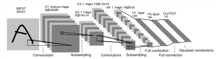
All the layers in the CNN are modelled around this image.

class CNN(nn.Module):
    def __init__(self):
        super(CNN, self).__init__()
        self.conv1 = nn.Conv2d(in_channels=1, out_channels=6, kernel_size=5)
        self.conv2 = nn.Conv2d(in_channels=6, out_channels=16, kernel_size=5)

        self.fc1 = nn.Linear(in_features=16 * 4 * 4,out_features=120)
        self.fc2 = nn.Linear(in_features=120, out_features=84)
        self.fc3 = nn.Linear(in_features=84, out_features=10)
    
    def forward(self, input):
        c1 = F.relu(self.conv1(input))
        s2 = F.max_pool2d(c1, kernel_size=2, stride=(2,2))
        c3 = F.relu(self.conv2(s2))
        s4 = F.max_pool2d(c3, kernel_size=2, stride=2)
        s4 = torch.flatten(s4, 1)
        f5 = F.relu(self.fc1(s4))
        f6 = F.relu(self.fc2(f5))

        output = self.fc3(f6)

        return output

import torch.nn.functional as F
F.max_pool2d(c1, kernel_size=2, stride=(2,2))
- This performs maxpool operation.
nn.Conv2d(in_channels=1, out_channels=6, kernel_size=5)
- This is used to perform convolution process.
torch.flatten(s4,1) or torch.flatten(torch.flatten(s4, start_dim=1)
- s4 is a 4D tensor with shape (batch_size, channels, height, width) or (N, C, H, W)
- start_dim=1 : function will flatten the tensor starting from dim=1 onwards.
  - preserves the first dimension.
  - flattens all remaining dimensions (C, H, W) into a single dimension.
- This function flattens the tensor s4 starting from dimension 1 onwards, converting a multi-dimensional tensor into a 1D vector per batch instance.
Trained the model using
- criterion = nn.CrossEntropyLoss()
- optimizer = optim.Adam(model.parameters(), lr=0.001)

Output

Epoch [1/20], Loss: 0.0830
Epoch [2/20], Loss: 0.0047
Epoch [3/20], Loss: 0.0095
Epoch [4/20], Loss: 0.0217
Epoch [5/20], Loss: 0.0113
Epoch [6/20], Loss: 0.0016
Epoch [7/20], Loss: 0.0001
Epoch [8/20], Loss: 0.1295
Epoch [9/20], Loss: 0.0002
Epoch [10/20], Loss: 0.0373
Epoch [11/20], Loss: 0.0004
Epoch [12/20], Loss: 0.0016
Epoch [13/20], Loss: 0.0010
Epoch [14/20], Loss: 0.0002
Epoch [15/20], Loss: 0.0006
Epoch [16/20], Loss: 0.0009
Epoch [17/20], Loss: 0.0014
Epoch [18/20], Loss: 0.0092
Epoch [19/20], Loss: 0.0000
Epoch [20/20], Loss: 0.0004

Accuracy: 98.92%

The full python code can be accessed here

Colab Notebook of the above code can be accessed here

Trained model parameters can be accessed here

Thus, CNN architecture and its implementation using PyTorch is performed.

Architecture

Convolutional Layer

Paramenters of Convolutional layer

1. kernel_size

2. stride

3. padding

4. dilation

5 in_channels & out_channels

Some terms regarding CNNs

1. Parameter Sharing

2. Receptive Field

3. Local Connectivity

Pooling Layers

Types of Pooling

Max Pooling

Average Pooling

Fully Connected Layer

PyTorch Implementation

Output

1. `kernel_size`

2. `stride`

3. `padding`

4. `dilation`

5 `in_channels` & `out_channels`