7. Computer Vision: Instance Segmentation
- Instance Segmentation involves classifying each pixel or voxel of a given image or volume to a particular class and assigning a unique identity to the pixels of individual objects.
- In Semantic Segmentation all objects belonging to a single class are assigned the same label without differentiating between different objects.
- In Instance Segmentation, the outline of objects, their spatial distribution matter, and individual identities are captured.
-
Is is a combination of object detection (class-wise localization) and segmentation (pixel-wise classification).
- Mask R-CNN is used for instance segmentation tasks.
Mask R-CNN
Components of Mask R-CNN :
1. Backbone Network
- A CNN to extract feature map from image.
- eg. ResNet-50
2. Region Proposal Network (RPN)
- Same as Faster R-CNN
- Check Here
3. RoI Align
-
Problem with RoI Pooling :
- it quantizes coordinates, causing misalignments.
- when dividing the region proposal into fixed size grid, it would round coordinates to nearest integers.
- this misalignments dropped accuracy.
4. Head Networks
| Branch | Task | Output | Loss |
| Classification | What class is it? | \(p \in \mathbb{R}^{K+1}\) (K classes + background) | Cross-entropy loss |
| Bounding box regression | Where is it exactly? | \(t \in \mathbb{R}^{4K}\) (4 for each class) | Smooth L1 loss |
| Mask prediction | Pixel-wise object mask | Binary mask of size m×mm \times mm×m per class | Per-pixel binary cross-entropy loss |
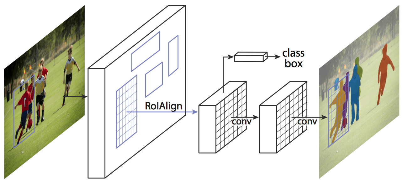
RoI Align
Steps :
- Take the RoI in floating-point coordinates.
- Divide the RoI into (eg.) 7×7 bins.
- In each bin, pick precise sample points (no rounding).
- Use bilinear interpolation to compute feature map values at those points.
- Aggregate (take average, max) to get the final feature for that bin.
Example
- Let a feature map be :
| y\x | 0 | 1 | 2 | 3 |
|---|---|---|---|---|
| 0 | 1 | 2 | 3 | 4 |
| 1 | 5 | 6 | 7 | 8 |
| 2 | 9 | 10 | 11 | 12 |
| 3 | 13 | 14 | 15 | 16 |
Image Coordinates : (0,0) is treated as the top-left pixel, and the y-axis values (row index) increase downwards.
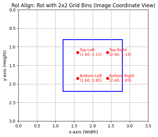
- Let the Region of Interset (RoI) be :
- Top-Left = (1.2, 0.8)
- Bottom-right = (2.8, 2.2)
-
Thus, the RoI has floating point coordinates
- Dividing the RoI into a grid :
- If the RoI feature pool to a 2x2 grid
- then RoI is divided into 4 bins.
- Width = 2.8 - 1.2 = 1.6
-
Height = 2.2 - 0.8 = 1.4
- Bin width = 1.6/2 = 0.8
- Bin Height = 1.4/2 = 0.7
- If the RoI feature pool to a 2x2 grid
-
Calculate the center of each of the bins :
-
-
Each of the red points are the center of their respective bins.
-
Using bilinear interpolation at each center point
- eg. For top-left bin center (1.6, 1.15):
- 4 nearest grid points :
(1,1) , (1,2), (2,1) & (2,2). - Values at these points =
[6, 7, 10, 11]
- 4 nearest grid points :
- Find
dx&dy:- dx = 1.6 - 1 = 0.6
- dy = 1.15 - 1 = 0.15
- Bilinear interpolation :
V = (1-dx)(1-dy)A + dx(1-dy)B + dy(1-dx)C + dxdyD- A : value at bottom-left corner.
- B : value at bottom-right corner.
- C : value at top-left corner.
-
D : value at top-right corner.
- dx = x − x1 : normalized horizontal distance between the interpolation point (x,y) and the left edge of the rectangle.
- measures how far the point is from the left side of the rectangle (range from 0 to 1).
- dy = y - y1 : normalized vertical distance.
- measures how far the point is from the bottom of the rectangle.
V = 7.2=Interpolated feature value at (1.6, 1.15)
- Bilinear interpolation considers the four nearest integer coordinate locations in the feature map to the sampling point.
- Then calculate a weighted average of the feature values at these four locations.
- The weights assigned to each neighbor are inversely proportional to the horizontal and vertical distances between the sampling point and that neighbor.
- Closer neighbors have a greater influence on the interpolated value.
- Allows to obtain feature values at sub-pixel locations, avoiding the information loss inherent in simply selecting the value at the nearest integer coordinate.
- Repeating for other 3 bins will give the 2x2 feature map for the RoI.
- If multiple were sampled per bin then take their average or max to summarize into a single feature value for that bin.
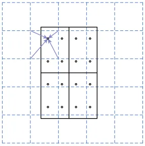
- dashed grid = feature map
- solid lines = RoI with 2x2 bins
- 4 sampling points in each bin
- Compute the value of each sampling point using bilinear interpolation from the nearby grid points on the feature map.
- Aggregate the result using avg. or max. to get a single representative value.
- Output is a feature map for each RoI.
- Repeating this for all RoIs.
- These feature maps are sent into 3 parallel head :
1. Classification head
- Predicts the class of the object
- Ouput : Class scores (softmax)
2. Bounding Box Regression head
- Refines the RoI (like in Faster R-CNN)
- Output : Bounding box adjustments
3. Mask head
- Predicts a pixel-wise binary mask for the object
- Output : A small 2D mask (eg. 28×28)
Mask Head
- small convolutional network added on top of the RoI features in Mask R-CNN.
- predict a pixel-wise segmentation mask inside each proposed RoI.
- tells which pixel belong to object or to background
- Mask head applies several convolutional layers to preserve spatial details.
- 4 conv layers of kernel size 3 with padding 1
- 1 deconvolution layer (upsampling) to increase size (14x14 -> 28x28)
- Finally a 1x1 Conv layer to output K masks. (one per class)
- Each masks is :
- 28x28 resolution
- Binary masks
- Each masks is :
-
Loss
- \(M_{pred}\) = predicted masks.
-
\(M_{gt}\) = ground truth binary masks.
- For each pixel apply binary cross-entropy loss between predicted mask and ground-truth mask:
- Loss = \(-[M_{gt}log(M_{pred}) \, + (1-M_{gt})log(1-M_{pred})]\)
- Sum it over all pixels inside RoI.
- Total Loss = L = \(L_{cls} \, + \, L_{bbox} \, + \, L_{mask}\)
Implementation in PyTorch
model = torchvision.models.detection.maskrcnn_resnet50_fpn(
    weights=torchvision.models.detection.MaskRCNN_ResNet50_FPN_Weights.DEFAULT
)
_ = model.eval()
- Rest is almost same as object detection code.
Colab Notebook with the complete implementation can be accessed here