NLP: Attention

What is the need of Attention?

In seq2seq models the encoder has to compress the whole soruce sequence into a single context vector. It is difficult for encoder to compress all the information about input sequence into a single context vector. At each generation step, different parts of source can be more useful than others. But the decoder has only access to same fixed context vector. This is a major bottleneck, that the netowrk is not able to remember long term dependencies. Attention mechanism tries to solve it by allowing the model to focus on the currently most relevant part of the source sentence.

What is Attention?

Introduced in the paper (Bahdanau et al., 2015), decoder uses a dynamic context vector $ c_i $ for each target word $ y_i $ it generates.

This $ c_i $ is a weighted sum of the encoder’s hidden states (annotations) from all source words.
There are many forms of Attention, here we will discuss Bahdanau Attention or Additive Attention.

from torch.nn.utils.rnn import pack_padded_sequence, pad_packed_sequence

Encoder Architecture

This is a bi-directional RNN. We will use a bi-directional GRU (GRU = Gated Recurrent Unit).
The Enocder (bidirectional GRU) : $ h_i = \left[ \overrightarrow{h}_i \, ; \, \overleftarrow{h}_i \right] $

I have used RNN and GRU interchangeably here. Both mean a Gated Recurrent Unit (GRU).

class Encoder(nn.Module):
  def __init__(self, input_size, hidden_size, num_layers = 1, dropout = 0):
    super(Encoder, self).__init__()
    self.num_layers = num_layers
    self.rnn = nn.GRU(input_size, hidden_size, num_layers, batch_first=True, bidirectional=True, dropout=dropout)

  def forward(self, x, mask, lengths):
    packed = pack_padded_sequence(x, lengths, batch_first=True)
    output, final = self.rnn(packed)
    output, _ = pad_packed_sequence(output, batch_first=True)

    fwd_final = final[0:final.size(0):2]
    bwd_final = final[1:final.size(0):2]
    final = torch.cat([fwd_final, bwd_final], dim=2)

    return output, final

Explanation of Encoder code :

```
self.rnn = nn.GRU(input_size, hidden_size, num_layers, batch_first=True, bidirectional=True, dropout=dropout)
```
- batch_first=True : The input and output tensors will have shape (batch, seq_len, feature)
- dropout : Used to set the dropout probability between layer

```
def forward(self, x, mask, lengths):
```
- x : A batch of padded sequences of shape (batch, seq_len, input_size)
- mask : Used for ignoring padding in attention
- lengths : A list of actual (unpadded) lengths of each sequence

```
  packed = pack_padded_sequence(x, lengths, batch_first=True)
```
Padding is done when working with batches of variable-length sequences to make them the same length.
- Preprares the padded sequences for GRU.
- lengths : actual sequence lengths (i.e., up to where values are valid, rest are padding).
- It packs only the real values, discarding the paddings.
- It keeps track of batch_sizes, sorted_indices, and unsorted_indices.

Another argument enforce_sorted : If True (by default), sequences must be sorted in descending order of length. If False, PyTorch will internally sort them.

Why Sorting?

Let the data with padding (unsorted) be :

Seq 1 (len 3): [A, B, C, PAD, PAD]
Seq 2 (len 5): [D, E, F, G, H]
Seq 3 (len 2): [I, J, PAD, PAD, PAD]

After Sorting (Descending) it becomes :

Seq 2 (len 5): [D, E, F, G, H]
Seq 1 (len 3): [A, B, C, PAD, PAD]
Seq 3 (len 2): [I, J, PAD, PAD, PAD]

Now, when this mini-batch is packed nad processed by RNN :

Time step 1: Processes D, A, I (3 active sequences)
Time step 2: Processes E, B, J (3 active sequences). Seq 3 (shortest) ends.
Time step 3: Processes F, C (Now only 2 active sequences). Seq 1 ends.
Time step 4: Processes G (Now only 1 active sequence)
Time step 5: Processes H (1 active sequence). Seq 2 ends.

This allows the RNN to process only the active (unpadded) sequences.
The GPU operations work most efficienty on contiguous blocks of data.
When sequences are sorted by length, the pack_padded_sequence function can arrange the data in a way that, at each time step, all the active tokens are grouped together.

```
  output, final = self.rnn(packed)   
```
- A packed sequence is fed into a bi-directional GRU and 2 values are returned output & final.
- output
  - It contains the hidden state $h_t$ at each time step t from the last (topmost) layer.
  - In RNNs Output at time t = Hidden state $h_t$ at time t.
  - It will be in packed form since the input was also packed.
  - After unpacking :
    - Shape : (batch_size, max_seq_len, hidden_size * 2)
    - hidden_size * 2 because the GRU is bidirectional.
    - The output at each time step is the concatenation of the forward and backward GRU outputs at that time step.
- final
  - Final hidden states from each direction & layer.
  - Shape : (num_layers * num_directions, batch_size, hidden_size)
    - num_directions = 2 if bidirectional=True.
    - Since the num_layers=1 :
      - Shape is (2, batch_size, hidden_size).
        
        final[0] : Last hidden state from forward GRU.
        
        final[1] : Last hidden state from backward GRU.

```
  output, _ = pad_packed_sequence(output, batch_first=True)
```
- pad_packed_sequence : It is used to convert a packed sequence back into a padded tensor.
- It returns the padded sequence & a tensor with the original lengths of the sequences.
- Shape of output = (batch, seq_len, 2 * hidden_size)

```
  fwd_final = final[0:final.size(0):2]    # slices out every even-indexed hidden state
  bwd_final = final[1:final.size(0):2]    # slices out every odd-indexed hidden state
```
- final.shape = [2, batch_size, hidden_size]
- A slicing operation is being performed.
- final.size(0) = num_layers * num_directions.
  - Here slicing is done along the first dimension (0).
- Thus, fwd_final.shape = bwd_final.shape = (num_layers, batch_size, hidden_size).

```
  final = torch.cat([fwd_final, bwd_final], dim=2)
```
- Concatenate both the forward and backward hidden states along dim=2.
- Dimension 2 is hidden size dimension.

Returns:

output : hidden states at every time step.

It tells how much does the model know about each word/token.

final : last hidden states from each layer & bidirectional.

It is a summary of the entire sentence/sequence.

Bahdanau Attention

Before discussing the Decoder, we will see what Attention is. There are many different types of Attention, but here we will discuss Bahdanau Attention or Additive / MLP Attention.

It allows the decoder to look back at all encoder states and decide which positions in the source to focus on.
Encoder outputs = $ h_1, h_2, h_3, …, h_t $
- Each $ h_i $ contains information about input word i and its context.
Decoder’s hidden state is denoted as $ s_t $.

Alignment Model

An alignment function or energy function is defined as :

\[a(s_{t-1} , h_i) = \nu_{a}^T \, tanh(W_a \, s_{t-1} + U_a \, h_i) = \text align (s_{t-1}, h_i)\]

Inputs :
- $ s_{t-1} \in \mathbb{R}^D $ : It is a vector which denotes the decoder’s previous hidden state.
  - Shape = [D x 1]
- $ h_{i} \in \mathbb{R}^{2D} $ : It is a vector which denotes the encoder’s hidden state at source position i.
  - Shape = [2D x 1]
Linear Mapping :
- A single score also called energy $ e_{t,i} $ measures how well $ s_{t-1} $ and $ h_i $ match.
- $ W_a $ and $ U_a $ are 2 learnable weight matrix of shapes [D x D] and [D x (2D)] respectively.
  - They map $ s_{t-1} $ and $ h_i $ into a common D-dimensional space by matrix-vector multiplication.
Applying nonlinearity :
- $ W_a \, s_{t-1} $ and $ U_a \, h_i $ are added to produce a D dimensional vector.
- tanh() is applied to this sum.
Projection to a scalar (energy) :
- $ \nu_{a} \in \mathbb{R} $ is a learnable column vector.
- A single real-valued number called energy is produced.
- \[e_{t,i} = \nu_{a}^T \, [tanh(W_a \, s_{t-1} + U_a \, h_i)]\]

This is performed using a Multi Layer Perceptron [MLP].

Normalizing the energies :
- After computing $ e_{t,i} $ for every i = 1,…, $ T_x $, ($ T_x $ denotes the length of the source sequence), they are normalized with a Softmax over $ T_x $ positions.
- \[\alpha_{t,i} = \frac{exp(e_{t,i})}{\sum_{j=1}^{T_x} exp(e_{t,j})} \quad \text for \, i = 1,..,T_x\]
- $ \alpha_{t,i} $ is the attention weight
- $ \sum_{i = 1}^{T_x} \alpha_{t,i} = 1 $

Attention Weight : Measures how strongly the decoder at time t wants to focus on (or align with) the i-th source word.

Energy : Raw, unnormalized measure of similarity/relevance.

Computing the Context Vector
- $ c_t $ is the weigthed sum of all encoder hidden states
- \[c_t = \sum_{i=1}^{T_x} \alpha_{t,i} \, h_i \quad \in \mathbb{R}^{2D}\]
- $ c_t $ encodes which part of the source sentence the model should pay attention to when generating the t-th target word.

The Modern QKV (Query-Key-Value) Framework

The QKV framework has become the standard for describing attention mechanism. I will use an example of a library to explain it.

Keys : It is the index cards in a library’s card catalog.
- Each key summarizes one item [one encoder time step].
Values : Actual information that is retrieved about that item.
- It is the full encoder hidden state at that position.
Query : It is the search request that the most relevant card to what I know currently is required.

Query : decoder’s current hidden state.

Key : encoder’s hidden state (compared against query to compute a similarity score).

Value : encoder’s hidden state (actual information retrieved used to form the context vector).

In Bahdanau attention, keys and values are the same.

Implementation

class BahdanauAttention(nn.Module):
    """Implements Bahdanau (MLP) attention"""
    
    def __init__(self, hidden_size, key_size=None, query_size=None):
        super(BahdanauAttention, self).__init__()
        
        # Determine dimensions for key vs. query if not passed explicitly.
        key_size   = 2 * hidden_size if key_size is None else key_size # shape of encoder hidden state
        query_size = hidden_size if query_size is None else query_size

        # Layers for projecting encoder “keys” and decoder “query” into a common space.
        self.key_layer   = nn.Linear(key_size, hidden_size, bias=False)
        self.query_layer = nn.Linear(query_size, hidden_size, bias=False)

        # Final “energy” layer that maps from the tanh output into a single scalar score.
        self.energy_layer = nn.Linear(hidden_size, 1, bias=False)
        
        # Placeholder to store computed attention weights (alphas).
        self.alphas = None

    def forward(self, query=None, proj_key=None, value=None, mask=None):
        assert mask is not None, "mask is required"

        # Project the decoder’s query into hidden_size space:
        query = self.query_layer(query)
    
        # Compute raw “energies” (scores) via an MLP followed by a linear “energy_layer”:
        scores = self.energy_layer(torch.tanh(query + proj_key))
        scores = scores.squeeze(2).unsqueeze(1)
        
        # Mask out padding positions in the source:
        scores.masked_fill_(mask == 0, -float('inf'))
        
        # Convert scores into normalized attention weights via softmax:
        alphas = F.softmax(scores, dim=-1)
        self.alphas = alphas        
        
        # Compute the context vector as weighted sum of values:
        context = torch.bmm(alphas, value)
        
        # Return both the context vector and the attention weights.
        return context, alphas

Explanation :

mask : It is a binary tensor that indicates which positions in a sequence should be attended to (1) and which should be ignored (0).
- The mask ensures attention doesn’t focus on these meaningless padding positions.
- If mask[i, j] == 0, that means “in batch example i, encoder position j is padding.
proj_key : [projects keys] It is the same thing as $ U_a \, h_i $ discussed above.
- It is initialized below in the decoder class as : proj_key = self.attention.key_layer(encoder_hidden).
query = self.query_layer(query) : It is the $ W_a \, s_{t-1} $ discussed above.
- Transforms the shape from : [batch, 1, query_size] to [batch, 1, hidden_size].
scores = scores.squeeze(2).unsqueeze(1) :
- Shape of scores = [batch, M, 1] (M = src_len).
- The shape is transformed to [batch, M] and then [batch, 1, M]
scores.masked_fill_(mask == 0, -float('inf'))
- Fills the element of the score tensor where value of mask is 0 with $ - \infty $.
- This happens only at padded positions.
- So when passed to softmax, $ exp(- \infty) \approx 0 $.
- So the model will never attend to paddings.
context = torch.bmm(alphas, value)
- bmm = Batch-Matrix-Multiplication
- Shape of alphas : [batch, 1, M]
- Shape of value : [batch, M, value_dim]
- For each example in the batch, it multiplies the 1×M row of attention weights by the M×value_dim matrix of encoder hidden states.

Decoder Architecture

class Decoder(nn.Module):
    def __init__(self, emb_size, hidden_size, attention, num_layers=1, dropout=0.5, bridge=True):
        super(Decoder, self).__init__()
        self.hidden_size = hidden_size
        self.num_layers = num_layers
        self.attention = attention
        self.dropout = dropout

        self.rnn = nn.GRU(
            emb_size + 2 * hidden_size, # Concatenated word embedding and context vector
            hidden_size, 
            num_layers, 
            batch_first=True, # inputs are (batch, seq, features)x
            dropout=dropout
            )

        self.bridge = nn.Linear(2 * hidden_size, hidden_size, bias=True) if bridge else None
        '''
        It is used to Convert the (2* hidden_size)-dimensional encoder summary into a 
        hidden_size-dimensional starting state for the decoder.
        '''

        self.dropout_layer = nn.Dropout(p=dropout)

        self.pre_output_layer = nn.Linear(hidden_size + 2 * hidden_size + emb_size, hidden_size, bias=False)
    
    def forward_step(self, prev_embed, encoder_hidden, src_mask, proj_key, hidden):

        # To perform a single decoder step, i.e., 1 word.

        query = hidden[-1].unsqueeze(1)

        context, attn_probs = self.attention(
            query=query,
            proj_key=proj_key,
            value=encoder_hidden,
            mask=src_mask
        )
        
        rnn_input = torch.cat([prev_embed, context], dim=2)
        '''
        prev_embed: (batch, 1, emb_size)
        context:    (batch, 1, 2*hidden_size)
        cat : (batch, 1, emb_size + 2*hidden_size)
        '''

        # run the GRU for one step
        output, hidden = self.rnn(rnn_input, hidden)

        pre_output = torch.cat([prev_embed, output, context], dim=2)
        pre_output = self.dropout_layer(pre_output)
        pre_output = self.pre_output_layer(pre_output)

        return output, hidden, pre_output

    def forward(self, trg_embed, encoder_hidden, encoder_final, src_mask, trg_mask, hidden=None, max_len=None):

        # unrolls the decoding process over all time steps

        if max_len is None:     # decides how many steps to run rnn
            max_len = trg_mask.size(-1)
        
        if hidden is None:
            hidden = self.init_hidden(encoder_final)
        
        proj_key = self.attention.key_layer(encoder_hidden)

        decoder_states = []
        pre_output_vectors = []

        for i in range(max_len):
            prev_embed = trg_embed[:, i].unsqueeze(1)
            '''
            trg_embed : [batch, trg_len, emb_size]
            trg_emb[:, i] : [batch, emb_size]
            then, [batch, 1, emb_Size]
            '''
            output, hidden, pre_output = self.forward_step(prev_embed, encoder_hidden, src_mask, proj_key, hidden)
            decoder_states.append(pre_output)
            pre_output_vectors.append(pre_output)
        
        decoder_states = torch.cat(decoder_states, dim=1)
        # decoder_states : list of length of max_len of shape : (batch, 1, hidden_size)
        # Concatenated along dim=1 : (batch, max_len, hidden_size)
        pre_output_vectors = torch.cat(pre_output_vectors, dim=1)
        return decoder_states, hidden, pre_output_vectors
    
     def init_hidden(self, encoder_final):

        if encoder_final is None:
            return None
        
        return torch.tanh(self.bridge(encoder_final))

Explanation of Decoder code :

Some of the code is already explained using comments above.

```
  self.pre_output_layer = nn.Linear(hidden_size + 2 * hidden_size + emb_size, hidden_size, bias=False)
```
- It is used to combine the following 3 things after each GRU step :
  1. The embedding of previous target token (size = emb_size).
  2. GRU’s output at that step (size = hidden_size).
  3. The attention context vector (size = 2 * hidden_size).
forward_step method is used to perform a single decoder step.

```
  query = hidden[-1].unsqueeze(1)  
```
- hidden : It is the current hidden state of the decoder GRU.
  - Shape : [num_layers, batch_size, hidden_size]
- hidden[-1] : Last element along the first dimension.
  - It extracts the hidden state of the topmost RNN layer
  - Shape becomes : [batch_size, hidden_size]
- .unsqueeze(1) : Adds a dimension at position 1.
  - Shape becomes : [batch_size, 1, hidden_size]

This whole Attention Mechanism can be visualized through this image :

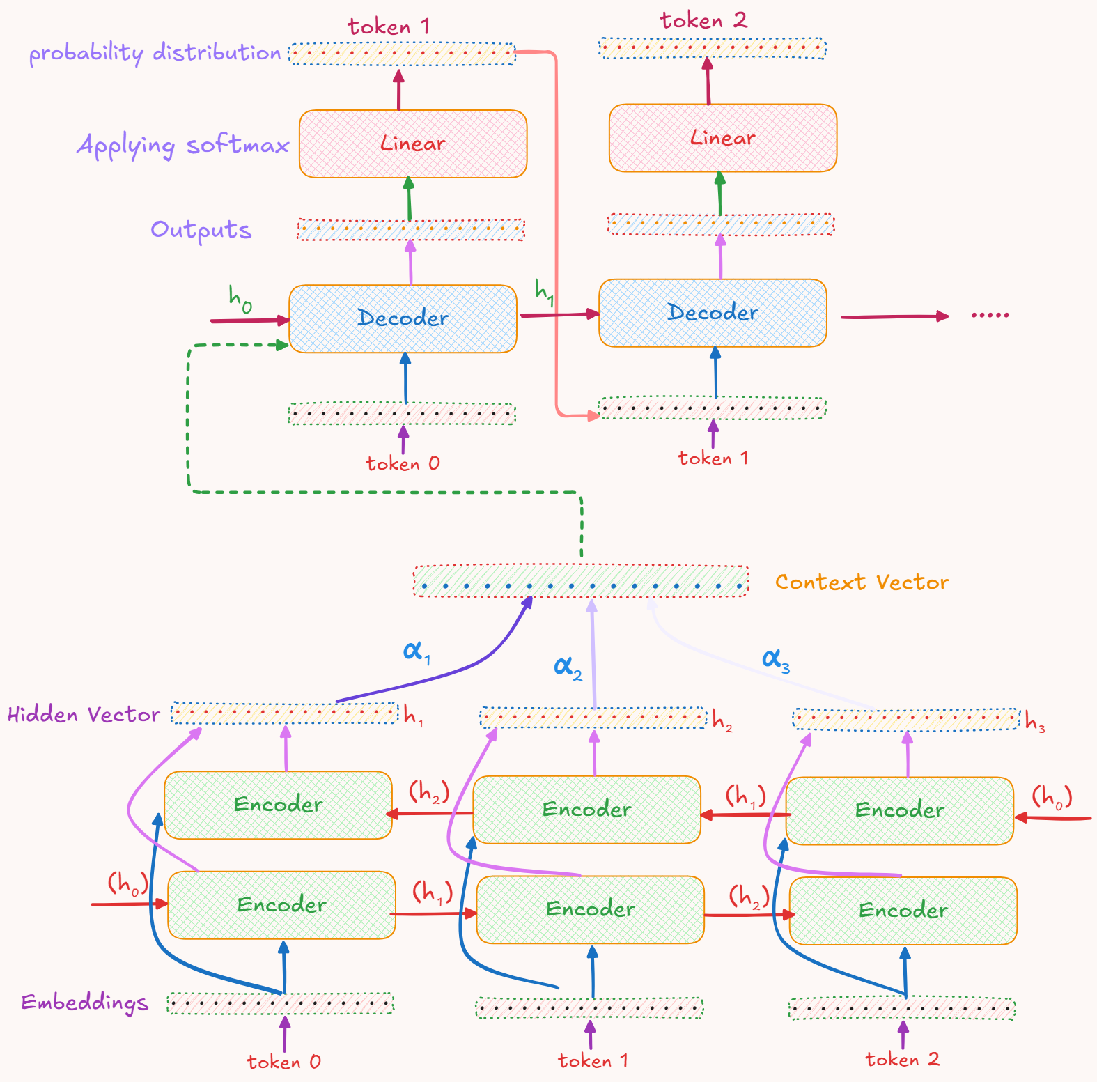
Now that all the components are ready, its time to group them together.

class EncoderDecoder(nn.Module):
    def __init__(self, encoder, decoder, src_embed, trg_embed, generator):
        super(EncoderDecoder, self).__init__()
        self.encoder    = encoder
        self.decoder    = decoder
        self.src_embed  = src_embed
        self.trg_embed  = trg_embed
        self.generator  = generator

    def forward(self, src, trg, src_mask, trg_mask, src_lenghts, trg_lengths):
        encoder_hidden, encoder_final = self.encode(src, src_mask, src_lenghts)
        return self.decode(encoder_hidden, encoder_final, src_mask, trg, trg_mask)

    def encode(self, src, src_mask, src_lenghts):
        return self.encoder(self.src_embed(src), src_mask, src_lenghts)

    def decode(self, encoder_hidden, encoder_final, src_mask, trg, trg_mask, decoder_hidden=None):
        return self.decoder(self.trg_embed(trg), encoder_hidden, encoder_final, src_mask, trg_mask, hidden=decoder_hidden)

Now the pre_output_layer needs to be mapped to the vocabulary size.

class Generator(nn.Module):
    def __init__(self, hidden_size, vocab_size):
        super(Generator, self).__init__()
        self.proj = nn.Linear(hidden_size, vocab_size, bias=False)

    def forward(self, x):
        return F.log_softmax(self.proj(x), dim=-1)

It turns each decoder hidden vector into a probability distribution over all target tokens.

This whole process can be shown in this picture :

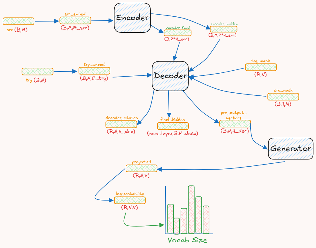
batch_size = B
src_len = M
trg_len = N
source_embedding_dim = E_src
target_embedding_dim = E_trg
encoder_hidden_size = H_enc (for each direction)
decoder_hidden_size = H_dec (for each layer; usually H_enc == H_dec)
vocab_size = V

Now the entire model is trained. This includes tokenization of the data, building a vocabulary, etc.
I have discussed these things in detail in the post Pytorch for NLP.

The complete implementation can be found here.

Visualizing Attention

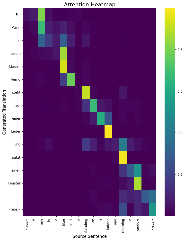
The color of each cell (x, y) shows how much attention the model paid to source word x when it was generating target word y. A brighter color means more attention.
Sharp Attention : A single bright yellow square for each target word shows the model is very confident.
Fuzzy Attention : If a row has several moderately bright squares, it means the model needed to look at a few source words to generate that target word (for complex phrases).

Beam Search

def beam_search_decode(model, src_tensor, src_mask, src_lengths, src_vocab, trg_vocab, beam_size=5, max_len=50, length_penalty=0.7):
    """
    Performs beam search decoding on a single sentence.
    
    Args:
        model: The trained EncoderDecoder model.
        src_tensor: A tensor of the source sentence IDs, shape (1, src_len).
        src_mask: The source mask tensor.
        src_lengths: The source lengths tensor.
        src_vocab: The source vocabulary object.
        trg_vocab: The target vocabulary object.
        beam_size (int): The number of hypotheses to keep at each step.
        max_len (int): The maximum length for the generated translation.
        length_penalty (float): Alpha factor for length normalization. 0=no penalty.
        
    Returns:
        A string representing the translated sentence.
    """
    model.eval()

    sos_idx = trg_vocab.stoi['<sos>']
    eos_idx = trg_vocab.stoi['<eos>']

    with torch.no_grad():
        # 1. Encode the source sentence once
        encoder_hidden, encoder_final = model.encode(src_tensor, src_mask, src_lengths)
        proj_key = model.decoder.attention.key_layer(encoder_hidden)
        decoder_hidden = model.decoder.init_hidden(encoder_final)

        # 2. Initialize the beam
        # Each beam contains: (cumulative_log_prob, sequence_tensor, decoder_hidden_state)
        beams = [(0.0, torch.LongTensor([sos_idx]).to(device), decoder_hidden)]
        completed_hypotheses = []

        for _ in range(max_len):
            if not beams:
                break # All beams have finished

            all_candidates = []
            
            # 3. Expand each beam
            for score, seq, hidden in beams:
                # Get the last token of the current sequence
                last_token = seq[-1].unsqueeze(0).unsqueeze(0)
                
                # Run one step of the decoder
                prev_embed = model.trg_embed(last_token)
                _, new_hidden, pre_output = model.decoder.forward_step(
                    prev_embed, encoder_hidden, src_mask, proj_key, hidden)

                # Get log probabilities for the next word
                log_probs = model.generator(pre_output).squeeze(1)

                # 4. Get top-k next tokens and their log-probs
                top_k_log_probs, top_k_indices = torch.topk(log_probs, beam_size, dim=-1)

                for i in range(beam_size):
                    next_token_idx = top_k_indices[0, i].item()
                    token_log_prob = top_k_log_probs[0, i].item()
                    
                    new_score = score + token_log_prob
                    new_seq = torch.cat([seq, torch.LongTensor([next_token_idx]).to(device)])
                    
                    all_candidates.append((new_score, new_seq, new_hidden))

            # 5. Prune the beams
            # Sort all candidates by their score
            all_candidates.sort(key=lambda x: x[0], reverse=True)
            
            # Reset the beams list for the next time step
            beams = []
            
            for new_score, new_seq, new_hidden in all_candidates:
                # If a hypothesis ends in <eos>, it's complete.
                if new_seq[-1].item() == eos_idx:
                    # Apply length penalty and add to completed list
                    # score / (length^alpha)
                    final_score = new_score / (len(new_seq) ** length_penalty)
                    completed_hypotheses.append((final_score, new_seq))
                else:
                    # This is still an active beam, add it to the list for the next step
                    beams.append((new_score, new_seq, new_hidden))
                
                # We only need to keep `beam_size` total hypotheses (both active and completed)
                if len(beams) + len(completed_hypotheses) >= beam_size:
                    break
            
            # To ensure we don't just keep expanding the same top beam, we only keep `beam_size` active beams
            beams = beams[:beam_size]

        # 6. Select the best hypothesis
        # If no hypothesis completed, use the best one from the active beams
        if not completed_hypotheses:
            # Fallback to the best active beam
            if beams:
                best_score, best_seq, _ = beams[0]
                completed_hypotheses.append((best_score/len(best_seq)**length_penalty, best_seq))
            else:
                return "" # Return empty if no translation could be generated

    # Sort all completed hypotheses by their normalized score
    completed_hypotheses.sort(key=lambda x: x[0], reverse=True)

    # Get the sequence of the best hypothesis
    best_seq = completed_hypotheses[0][1]
    
    # Convert token IDs to words
    trg_tokens = [trg_vocab.itos[idx.item()] for idx in best_seq]
    
    # Return translation, excluding <sos> and <eos>
    return " ".join(trg_tokens[1:-1] if trg_tokens[-1] == '<eos>' else trg_tokens[1:])

Beam Search can be visualised through this diagram :

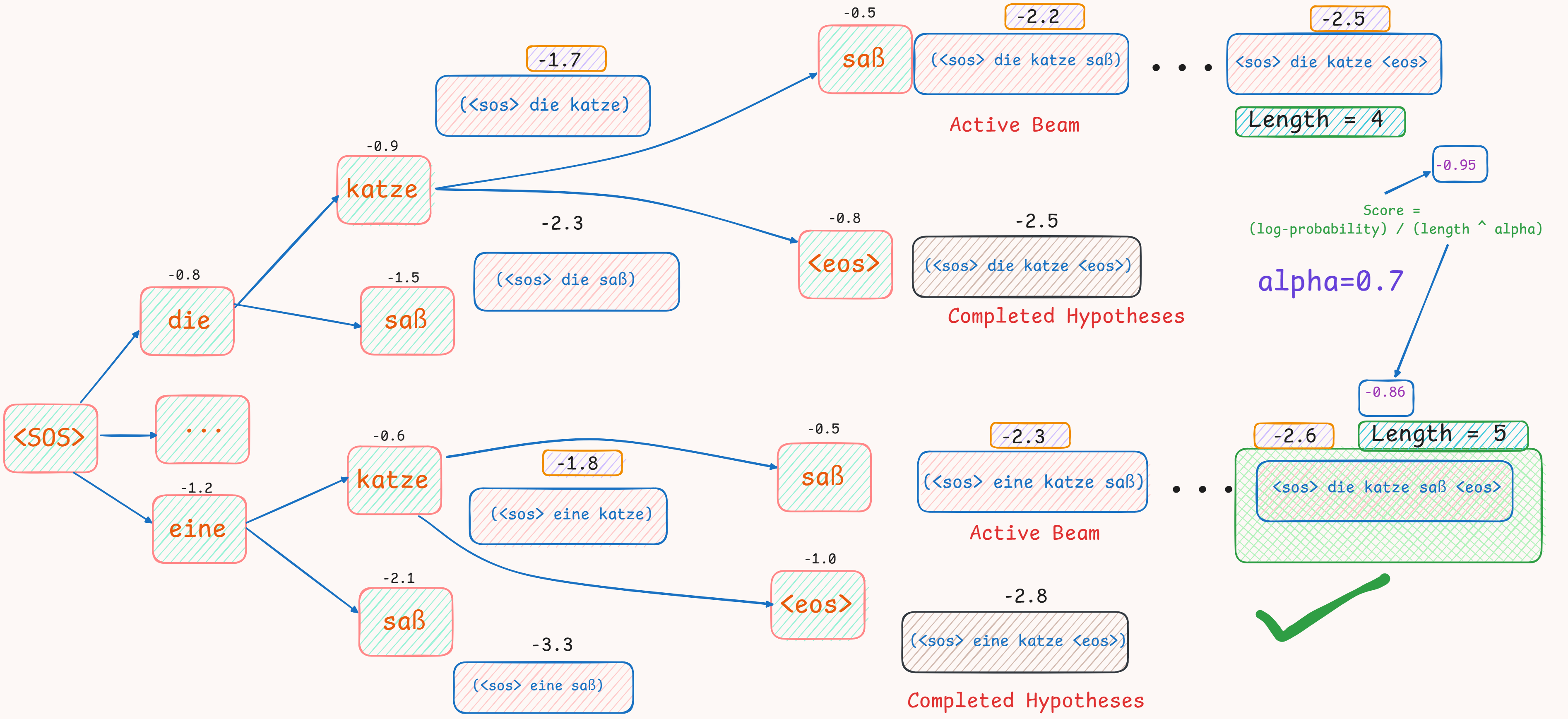
Here :
- Source Sentence: “the cat sat”
- Beam Size (k): 2
- The final score (after length normalization) is calculated as : $ \frac{raw \, score}{\alpha^{\text length}} $.

5. NLP: Attention

What is the need of Attention?

What is Attention?

Encoder Architecture

Explanation of Encoder code :

Why Sorting?

Bahdanau Attention

Alignment Model

Inputs :

Linear Mapping :

Applying nonlinearity :

Projection to a scalar (energy) :

Normalizing the energies :

Computing the Context Vector