Attention Is All You Need Deep Dive

Transformer architecture was introduced in the paper “Attention is All You Need” by Vaswani et al. in the year 2017. Transformers allowed to understand the relationships between all parts of an input parallelly. This allowed much faster training, better performance, and superior handling of complex tasks like language translation, summarization, and text generation than previous models/architectures like RNNs or LSTMs.
Transformers are the backbone of all the modern AI advancement. From language modelling to vision all the SOTA (State Of The Art) models utilize transformers.

This post will be broken down into the following subparts :

Background
Transformer Architecture Overview
Position-wise fully connected feed-forward network
Scaled Dot-Product Attention
Multi-Head Attention
Masked Multi-Head Attention (MHA)
Types of MHA Used
Embedding & Positional Encoding

1. Background

Recurrent Neural Networks (RNNs) process the input sequence token-by-token which doesn’t allow for parallelization. This makes the training process slow.
RNNs tend to forget distant context due to vanishing gradients (even with LSTMs and GRUs). This makes them unreliablle for understanding long sequences.
CNNs (Convolutional Neural Network) are parallelizable but they also struggle to model dependencies between distant tokens.
Attention models (like Bahdanu and Luong Attention) were imporoving tasks like translation and summarization.
The Transformer architecture took the idea of attention and made it the core component, eliminating the need for recurrence or convolutions entirely.

2. Transformer Architecture Overview

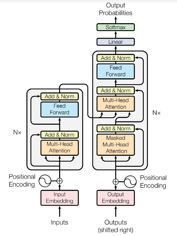
The model consists of an encoder and a decoder.

Encoder

The encoder consists of a stack of 6 identical layers, which inturn consists of 2 sub-layers (from bottom to top) :
1. Multi-head-self-attention mechanism
2. Position-wise fully connected feed-forward network

A residual connection is applied around each of the 2 sub-layers, follwed by layer normalization.

Residual Connection

It is a shortcut path that bypasses a layer and adds the input of the layer directly to its output.
So, if $ F(x) = \text{SelfAttention}(x) \, or \, F(x) = \text{FFN}(x) $ , with $ x $ being the input to the sublayer $ F(x) $ , then :

\[\text{Sum} = x + F(x)\]

So, the input goes into the sublayer and also around it via the residual connection (Skip Connection).
It allows the model to preserve information through the layers and learn only the difference (residual).

Layer Norm

Before understanding Layer Norm it is important to undersatnd why it is needed.

Internal Covariate Shift

It is the phenomenon where the inputs to a layer (activations) keep changing as the parameters of the previous layers update during training.
This causes each layer to constantly adapt to new input distributions which causes learning to be slow and unstable.
Gradient descent struggles because it keeps chasing a moving target.
It is used to normalize the activations across the features of a single data point.

Let $x$ ( of shape [batch size, feature dimension] ) be the batch of inputs to the network :

$x = \begin{bmatrix} x_{11} & x_{12} & \cdots & x_{1H} \\ x_{21} & x_{22} & \cdots & x_{2H} \\ \vdots & \vdots & \ddots & \vdots \\ x_{B1} & x_{B2} & \cdots & x_{BH} \end{bmatrix}$

Then,
- Each row $ x_i \in \mathbb{R}^{H} $ is a single data point.
- Each column represents a feature
Layer Norm operates on each row independently.
For each data point $ x = [x_1,x_2,\dots,x_H] $ (H = number of hidden units (features)), Layer Norm computes :
- Mean :
  - \[\mu = \frac{1}{H} \sum_{i=1}^H x_i\]
- Variance :
  - \[\sigma^2 = \frac{1}{H} \sum_{i=1}^H (x_i - \mu)^2\]
- Normalize :
  - \[\hat x_i = \frac{x_i - \mu}{\sqrt{\sigma^2 + \epsilon}}\]
- Scale & Shift :
  - \[y_i = \gamma_i \hat x_i + \beta_i\]
$ \gamma $ & $ \beta $ are learnable parameters and are of same size as x.
$ \epsilon $ is a small constant to avoid division by 0.
Nerworks train better and faster when the inputs to each layer have 0 mean and unit variance.
Layer Norm helps in stabilizing learning and improves convergence speed.

Thus, the flow of operations for each sublayer is like :

\[\text{Output}_1 = \text{LayerNorm} (x + \text{SelfAttention}(x))\] \[\text{Output}_2 = \text{LayerNorm} (\text{Output}_1 + \text{FFN}(\text{Output}_1))\]

The outputs of each sub-layer as well as the embedding layer are of the same dimensions. In the paper it was $ d_{model} $ = 512.

Decoder

Decoder is also very similar to the Encoder.
It consists of a stack of 6 identical layers.
Each layer consists of 3 sub-layers (from bottom to top) :
1. Masked Multi-Head Attention
2. Multi-Head Attention (over the output of the encoder stack)
3. Position-wise fully connected feed-forward network
And just like in Encoder here also residual connections are employed around each sub-layer followed by layer normalization.

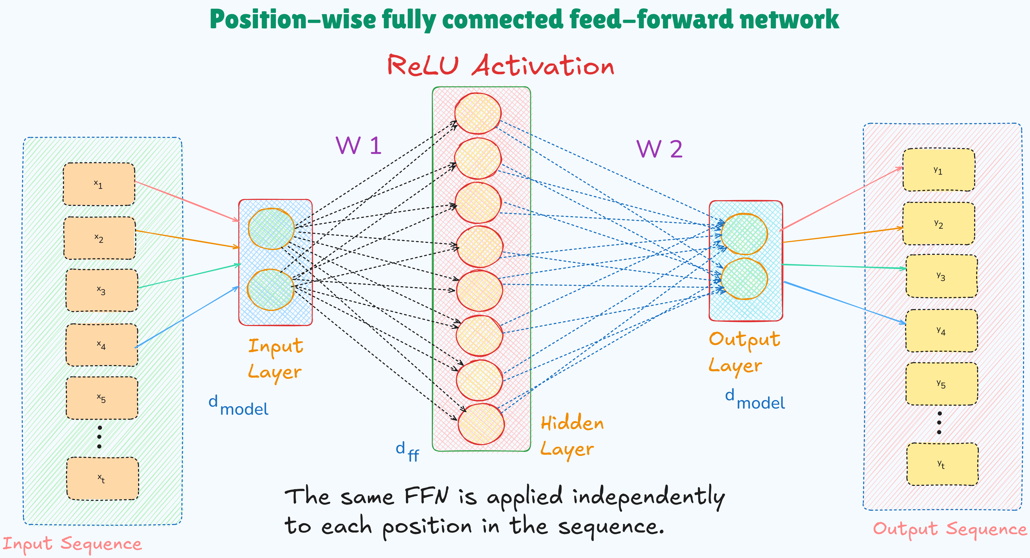
3. Position-wise fully connected feed-forward network

It is a 2 layer MLP (Multi Layer Perceptron) applied independently to each position (token vector) in the input sequence.

\[\boxed{ \text{FFN}(x) = \max{(0, xW_1 + b_1)}W_2 + b_2 }\]

Where,
- $ x \in \mathbb{R}^{d_{model}} $ : It is the input vector (eg. 512-dimensional)
- $ W_1 \in \mathbb{R}^{d_{model} \times d_{ff}} $ : Weight matrix 1 (eg. $ d_{ff} = 2048 $)
- $ W_2 \in \mathbb{R}^{d_{ff} \times d_{model}} $ : Weight matrix 2
- $ b_1 $ and $ b_2 $ : Bias vectors
- $ \max{(0, \cdot)} $ : ReLU activation
This 2 layer MLP is applied at each position (token) vector independently / separately.
There is no interaction between tokens during this step and each token in processed using the same network.

It transforms each token’s representation individually allowing the model to re-map the token into a richer space (a (vector) space where token representations carry more complex and contextual information) after gathering context via the attention layer.

4. Scaled Dot Product Attention

Attention allows the model to dynamically focus on the different parts of the input sequence when processing each token. A weighted representation of the entire input sequence for each token is computed so that the model can selectively attend to the most relevant words. This information is captured using a usefulness score.

The concept of Queries, Keys, and Values is used to compute attention.
Consider a database which consists of some Key-Value pairs.
To retrieve information from the database a query is issued.
The given query is compared to all the keys stored in the database to compute similarity scores.
Based on these scores, the most relevant values are returned.

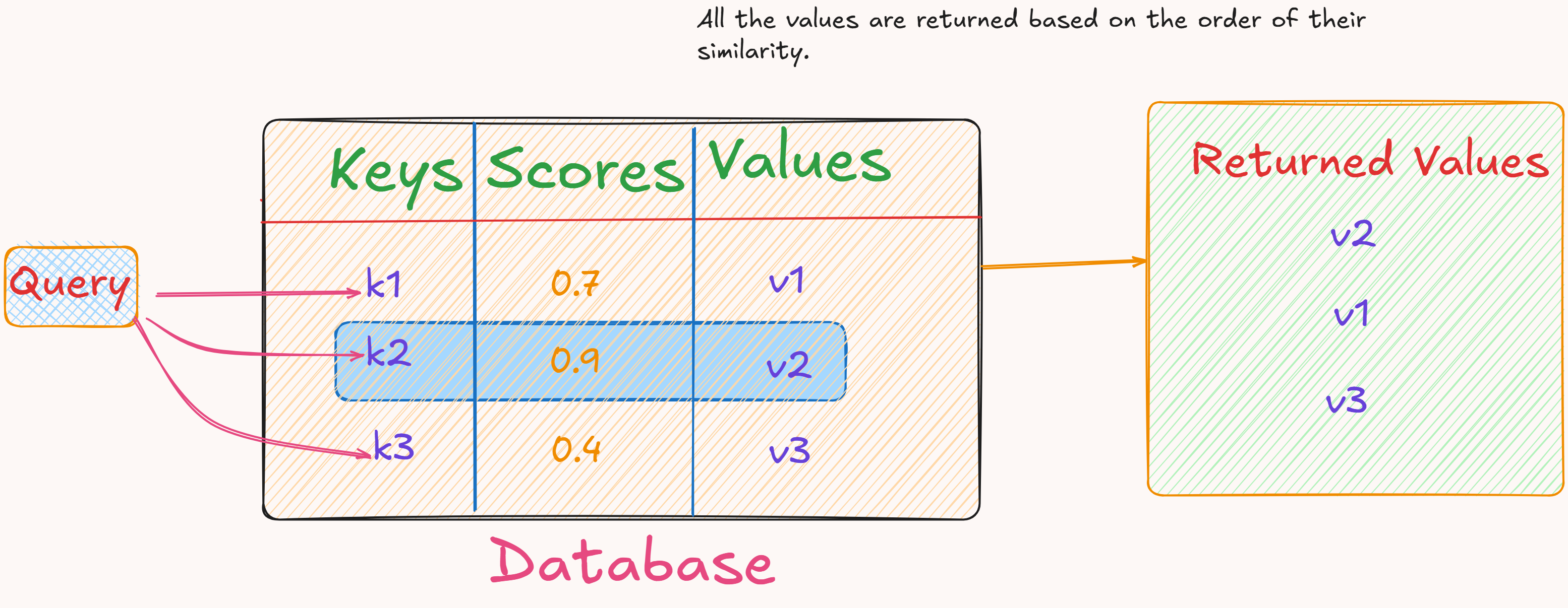
The above analogy can be used to understand Queries, Keys, and Values in context of attention.

To compute the attention of a word in one sentence with respect to all words in another sentence :

Create a Query vector for the word.

Create Key and Value vectors for each word in the second sentence.

Compute the similarity between the Query and each Key.

It gives the raw attention score for each word in the second sentence.

Pass the resulting scores through a softmax function, turning them into a probability distribution.

It converts the scores into a set of positive weights that all sum up to 1.

Each weight represents how much attention the query word should pay to each value.

Compute the weighted sum of all the value vectors using the softmax weights.

This results in a single output vector which is just the enriched version of the original word representation with relevant context from other sentence.

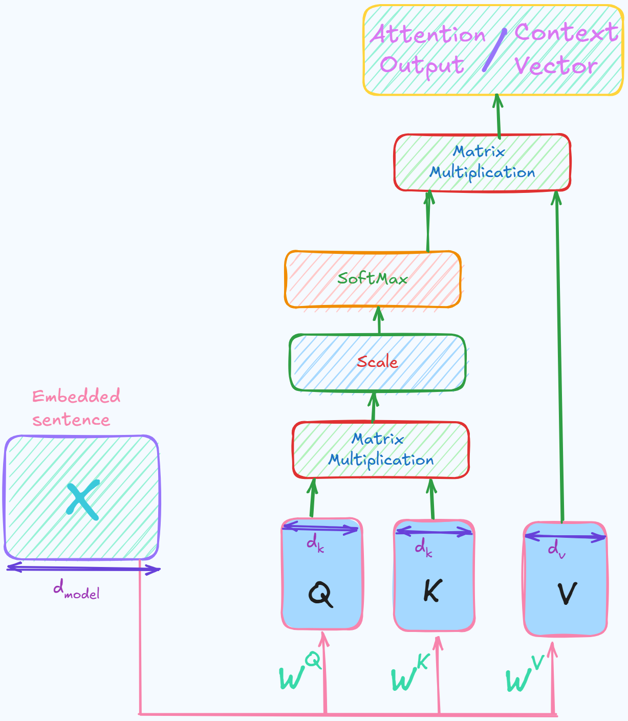
Mathematical formulation of Scaled Dot Product Attention

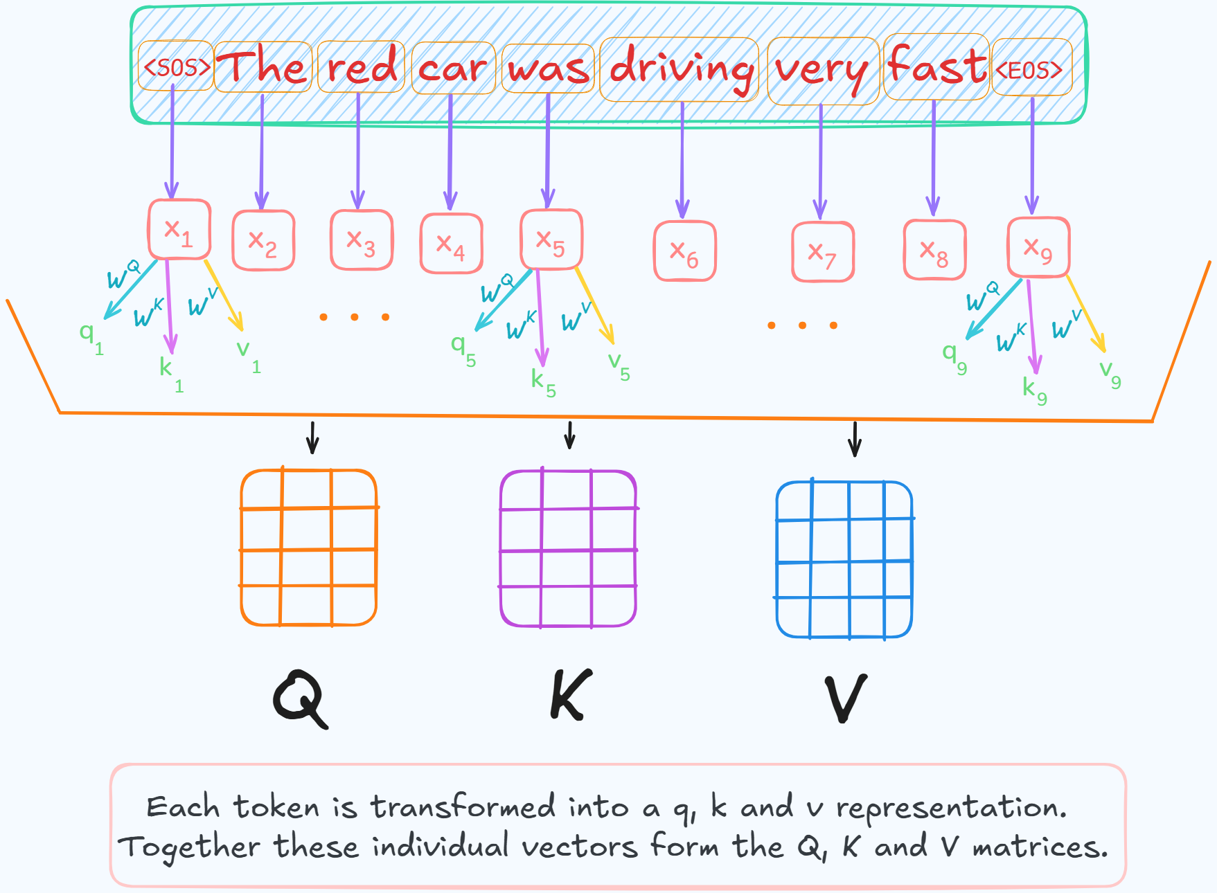
$ X = [x_1, x_2, \cdots, x_n] \in \mathbb{R}^{n \times d_{model}} $
- $ X $ is the matrix of all vectorized tokens in the input sequence of length $ n $ where each token is of dimensionality $ d_{model} $.
- $ x_i \in \mathbb{R}^{d_{model}} $ is the embedding vector of the $ i^{th} $ token.
To compute attention between these tokens, their vector embeddings are projected into 3 new vector spaces using learned matrices.

\[\boxed{ \begin{array}{rl} Q &= XW^Q \quad \text{(queries)} \quad \in \mathbb{R}^{n \times d_k} \\ K &= XW^K \quad \text{(keys)} \quad \in \mathbb{R}^{n \times d_k} \\ V &= XW^V \quad \text{(values)} \quad \in \mathbb{R}^{n \times d_v} \end{array} }\]

$ Q $, $ K $ & $ V $ are the linear transformations of $ X $.

$Q$ and $K$ are of same dimensionality as their dot product is calculate which requires them to be of same dimensionality.

$V$ can have different dimension because it is not used for any dot product calculation but for just weighted sum.

Where :
- $ W^Q \in \mathbb{R}^{d_{model} \times d_k} $
- $ W^K \in \mathbb{R}^{d_{model} \times d_k} $
- $ W^V \in \mathbb{R}^{d_{model} \times d_v} $
These are the learned parameters / weights of the model.
They may be of different dimensionalities.

The main idea behind scaled dot product attention mechanism is to :

Compare each query with all the keys to get attention weights.
Use these weights to compute a weighted sum over the values.

a. Dot Product

Similarity between the query and key is computed using their dot product. $ q \cdot k = \sum_{j=1}^d q_j k_j = \left\lVert q \right\rVert \left\lVert k \right\rVert \cos\theta $

If $ \cos\theta $ is 1 then the vectors are aligned and if they are orthogonal then it will be 0.

Thus, dot product increases with alignment and is considered unnormalized similarity measure.

Thus the attention scores are computed as :

\[\boxed{\text{scores} = QK^T \in \mathbb{R}^{n \times n}}\]

Where each element’s score [ $ scores_{ij} = q_i \cdot k_j $ ] represents how much each token $ i $ attends to token $ j $.

b. Scaling

Now the scores are scaled. If the dimensionality of the vectors is large (eg. $ d_k = 512 $), then the dot product can produce large values.
When these scores are passed through softmax function, the output will have one element get all the attention and others nearly 0.
This leads to vanishing gradients problem during training as very small gradients may be generated.

Thus the scores (dot product) is scaled by $ \sqrt{d_k} $ (square root of the key dimension).

\[\boxed{\text{scaled scores} = \frac{QK^T}{\sqrt{d_k}} }\]

c. Applying Softmax

$\text{softmax}(z)_i = \frac{\exp{z_i}}{\sum_{j=1}^N \exp{z_j}}$ function is applied row-wise, i.e. for each token $ i $, $ \alpha_i = \text{softmax}(\frac{q_i \cdot K^T}{\sqrt{d_k}}) $ is computed.

This gives a probability distribution over all n tokens in the sequence.
$ \alpha_{ij} $ tells how much attention token $i$ pays to token $j$.
Thus,

\[\boxed{ \alpha = softmax(\frac{QK^T}{\sqrt{d_k}}) \in \mathbb{R}^{n \times n} }\]

Each row of $\alpha$ matrix corresponds to one token’s attention distribution over all tokens in the sequence including itself.
Each row being a probability distribution sums to 1.
softmax returns a vector when a vector is passed to it but a matrix when a matrix is passed to it where each row is a softmaxed vector.

d. Multiply with Values

\[\boxed{ Attention(Q,K,V) = softmax(\frac{QK^T}{\sqrt{d_k}})V \in {n \times d_v}}\]

It is same as $\alpha V $.
Each row $\alpha_i$ is the attention distribution (weights) for token $i$ and $V$ contains the all the value vectors for all tokens (one per row).

Thus, $ \alpha_i V = \sum_{j=1}^n \alpha_{ij} v_j $ resembles computing a weighted sum of all the value vectors where weights are how much attention token $i$ pays to token $j$.

This gives a new vector representation for token $i$, which summarizes information from the whole sequence, weightd by attention.

5. Multi-Head Attention

Multi-head attention takes the scaled dot-product attention a step further by performing it multiple times in parallel with different learned linear projections of the queries, keys and values.
An Attention-Head is just one instance of performing scaled dot-product attention.
- It is just an attention layers.
- It focuses on learning a specific aspect or relationship in the data.
Multiple heads are used parallely, allowing each head to attend to different parts of the input representation space.
Let : $h$ : number of head (in the paper $h = 8$)
$ d_{model} $ : dimension of model
$ d_k = d_v = \frac{d_{model}}{h} $ : dimension of each head
$X$ : Layer Input of shape [batch_size, seq_len, d_model]
- eg. [32, 50, 512] (32 sentences, 50 tokens each, 512-dim embedding).

Reduced dimension of each head results in a similar total computation costs as that of single-head attention with full dimensionality.

But single attention head will not allow the model to jointly attend to information from different representation subspaces at different positions.

There are 2 ways to understand Multi-Head Attention (MHA).
Both ways are mathematically equivalent.
They differ in their computational arrangements.
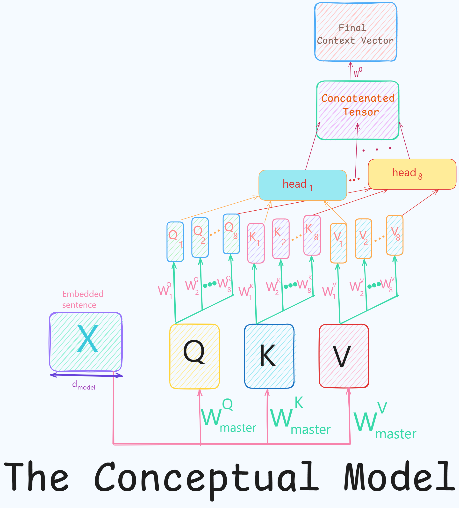
1. The Conceptual Model :
  - It is the same approach as mentioned in the original paper.
  - It explains the idea of multiple heads learning different feature representations in parallel.
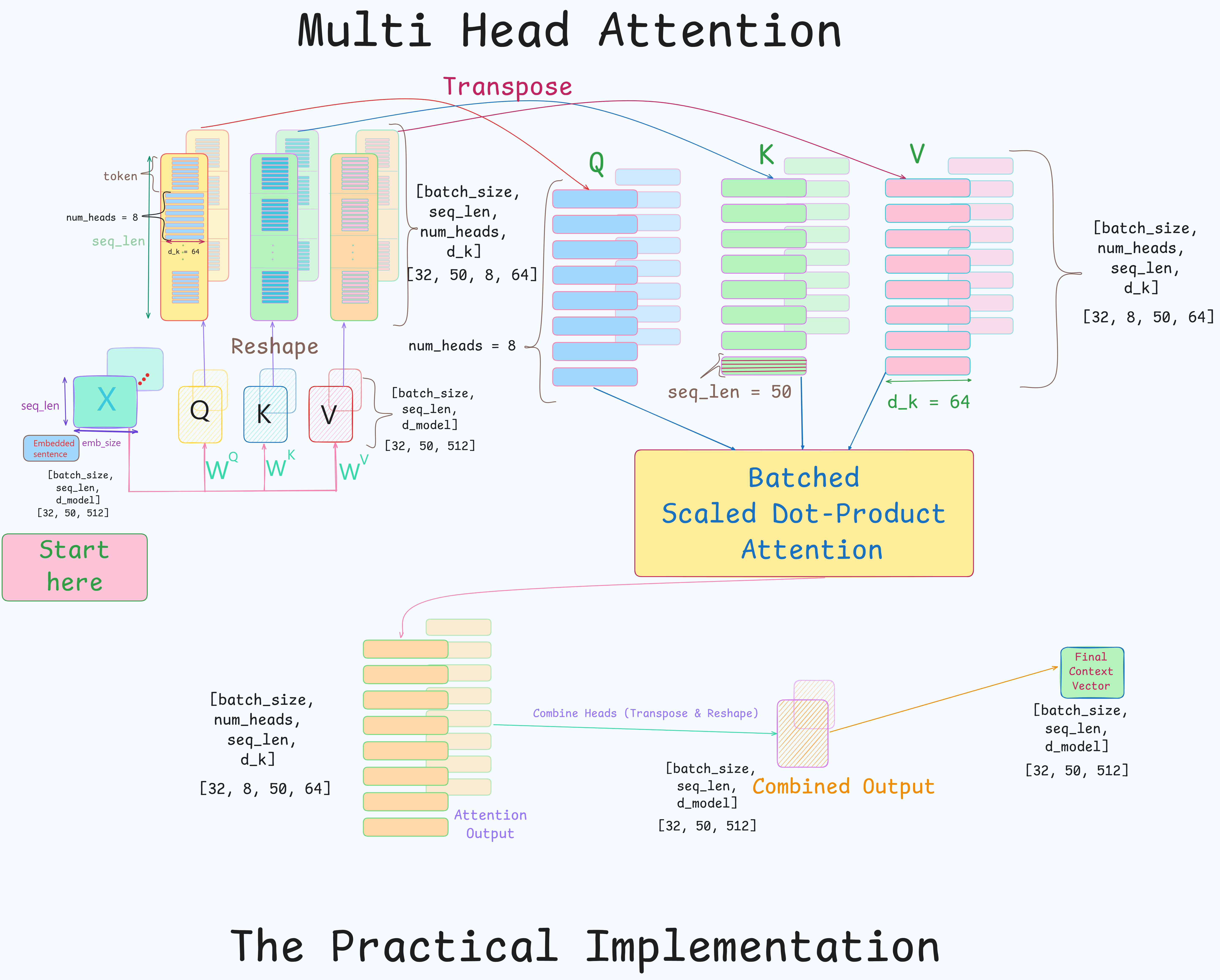
2. The Practical Implementation :
  - It is the optimized approach used in modern deep-learning libraries (PyTorch & TensorFlow).
  - It reframes the computation into a single, large, batched operation.
  - It is designed to be efficient on GPU hardware.

The Conceptual Model

This model follows a logic like : $ create \rightarrow split \rightarrow process $.

Create main / master $Q$,$K$,$V$ matrices and then for each head independently project these down to smaller dimension and then calculate attention.

1. Initial Generation of Master Q,K,V :

\[\begin{array}{rl} Q &= X W_{master}^Q \\ K &= XW_{master}^K \\ V &= XW_{master}^V \end{array}\]

The input embeddings $X$ are projected onto $Q,K,V$ matrices.
$W_{master}^y$ are learnable weight matrices each with a shape [d_model, d_model] (eg. [512, 512]).
Resulting $Q$,$K$,$V$ matrices are the inputs to the MHA each of shape : [batch_size, seq_len, d_model] (eg. [32, 50, 512]).

2. Split : [Head-specific Projections]

For each head $i$ a second set of learned linear projections are defined.
Weight matrices for each head $i$ : $W_i^Q, W_i^K, W_i^V$ are of shape [d_model, d_k] (e.g., [512, 64]).

\[\begin{array}{rl} Q_i &= QW_{i}^Q \\ K_i &= KW_{i}^K \\ V_i &= VW_{i}^V \end{array}\]

$Q$,$K$,$V$ matrices are projected through each head to create the inputs for that specific head.
Resulting shape of $Q_i$,$K_i$,$V_i$: [32, 50, 64].
This step is performed in parallel for all 8 heads.

3. Parallel Attention Calculation

\[head_i = Attention(Q_i,K_i,V_i) = softmax(\frac{Q_i K_i^T}{\sqrt{d_k}}) V_i\]

Each head independently calculates the attention score using its unique $Q_i, K_i, V_i$.
The output for each $head_i$ is a tensor of shape [32, 50, 64].

4. Concatenation and Final Projection

Outputs from all 8 heads are concatenated along the last dimension.
- (batch, seq, 64) $ \times $ 8 = (batch, seq, 512) = (32, 50, 512)
The concatenated tensor is passed through one last linear projection $W^O$ of shape [512, 512] to produce the final MHA output.

\[\text{MHA Output} = Concat(head_1, \cdots, head_8) W^O\]

The Practical Implementation

This model follows a logic like : $ project \rightarrow split $.

Perform one large projection that contains all head projections at once and then reshape the result to get the separate heads.

1. Fusing the projection steps

The projections steps (1 & 2 steps of the conceptual model) are combined into one.
One large weight matrix is used instead of multiple small weight matrices to compute $Q,K,V$.
Thus combined weight matrices of each head : $W^Q, W^K, W^V$ are used each with shape : [d_model, d_model] = [d_model, h * d_k] = [512, 512].
A single weight matrix does the job of $W_{master}$ and all the $W_i$ matrices from the conceptual model.
$Q_{all}$ or $Q$ and other 2 matrices are similarly computed :

\[\begin{array}{rl} Q' &= QW^Q \\ K' &= KW^K \\ V' &= VW^V \end{array}\]

From here on $Q’,K’,V’$ are written as $Q,K,V$

Each of these 3 tensors (matrices) are of shape : [32, 50, 512].

2. Reshape and Transpose for Heads [Split part]

Currently the tensors $Q,K,V$ are of shape [32, 50, 512] or [batch_size, seq_len, embed dim].
The last dimension is reshaped into [h, d_k].
- Thus, $Q,K,V$ become of shape : [32, 50, 8, 64] = [batch_size, seq_len, num_heads, dim_head]

Tensor Transpose : It is about swapping dimensions.

eg. Transpose(dim1, dim2). This will swap dimension 1 with 2.

Transpose(seq_len, num_heads) to group all heads together for batched computation.
- [32, 50, 8, 64] -> [32, 8, 50, 64] = [batch_size, num_heads, seq_len, dim_head].
- This is done for all 3 $Q,K,V$.

Reasoning behind transpose :

Exam Grading Analogy :

Let there be an exam in 32 sections. ([batch_size])

The exam consists of 8 questions. ([seq_len])

Teacher can check each student’s paper sequentially but it will be inefficient beacuse teacher will have to constantly switch context, i.e., logic of Q.1 then Q.2 and so on.

The better way will be to take all the Q.1s of all 8 students and group them in a pile and repeat the same for all the other 31 Questions.

Now, pick up a pile and grade all the 32 questions of that pile.

It will be quicker beacuse teacher will be in the same mindset.

That is grading is done as a batch operation, which GPUs are optimized for.

Applying this analogy to the projected tensor :
- Initial state :
  - [batch_size, seq_len, num_heads, dim_head]
  - [32 students, 50 words, 8 questions, 64 features per question]
- Now, traspose(1, 2) i.e., swap seq_len with num_heads :
- Resulting shape will be : [batch_size, num_heads, seq_len, dim_head] = [32 students, 8 questions, 512 words, 64 features per question]
- The deep learning libraries like PyTorch will see [batch_size, num_heads] dimensions as one large batch of task.

Another way to look at this :

Let batch_size = 2 (i.e. 2 sentences are being processed at once), seq_len = 3 and num_heads = 4.
Before transpose, let the data in memory be arranged like this :

// batch 1
Toeken A1 : [Head1_data, Head2_data, Head3_data, Head4_data]
Toeken A2 : [Head1_data, Head2_data, Head3_data, Head4_data]
Toeken A3 : [Head1_data, Head2_data, Head3_data, Head4_data]

//batch 2
Toeken B1 : [Head1_data, Head2_data, Head3_data, Head4_data]
Toeken B2 : [Head1_data, Head2_data, Head3_data, Head4_data]
Toeken B3 : [Head1_data, Head2_data, Head3_data, Head4_data]

If calculation for Head 1 is to be done, then GPU will have to take big jumps to access the data oh Head 1 from all the tokens.
The data is scattered all over memory.
After Transpose :

// batch 1
Head 1 : [Token A1_data, Token A2_data, Token A3_data]
Head 2 : [Token A1_data, Token A2_data, Token A3_data]
Head 3 : [Token A1_data, Token A2_data, Token A3_data]
Head 4 : [Token A1_data, Token A2_data, Token A3_data]

// batch 2
Head 1 : [Token B1_data, Token B2_data, Token B3_data]
Head 2 : [Token B1_data, Token B2_data, Token B3_data]
Head 3 : [Token B1_data, Token B2_data, Token B3_data]
Head 4 : [Token B1_data, Token B2_data, Token B3_data]

The library will see [batch_size, num_heads] dimensions as one large batch of task.
- That is, it will see 2 * 4 = 8 independent problems to solve and all the data it needs is in one block.

After transpose(1,2) the tensor can be considered as a batch of (batch_size, num_heads) individual matrices each of size (seq_len, dim_head).
This allows to perform a single, efficiet matrix multiplication that calculates the attection score for all heads and all sequences in the batch simultaneously.

3. Batch Scaled Dot-Product Attention Calculation

Now both $Q$ and $K$ have the same shape = [batch_size, num_heads, seq_len, dim_head].
$K$ will need to be transposed for computing scaled dot product attention.
- Last 2 dimensions of $K$ are transposed, resultant shape of $K^T$ : [batch_size, num_heads, dim_head, seq_len].
- This can be done using traspose(-2, -1).
  - This means to transpose / swap the last 2 dimensions.
Now $QK^T$ will result in attention score matrix of shape : [batch_size, num_heads, seq_len, seq_len].
- The matrix multiplication happens between the last 2 dimensions ([50, 64] & [64, 50]).
Thus, in each batch there is a [seq_len, seq_len] shape matrix showing how much each token attends to every other token.
After this the product is scaled by $\sqrt{d_k}$ which doesn’t change the shape.
Now the scaled dot-product is multiplied with $V$ which is of shape : [batch_size, num_heads, seq_len, dim_head].
- Resulting shape is : [batch_size, num_heads, seq_len, dim_head]

4. Reverse, Reshape and Final Projection (Concatenation):

The final output of the MHA layer which will be the input of the next layer (FFN) needs to be of shape [batch_size, seq_len, d_model].
To convert the current tensor :
1. Reverse the transpose.
2. Concatenate the Heads.
After traspose(1,2) shape will become : [batch_size, seq_len, num_heads, dim_head]
- ([32, 8, 50, 64] -> [32, 50, 8, 64]).
The concatenation of last 2 dimensions is done by reshape or view operation.
- eg. reshape(batch_size, seq_len, num_heads * dim_head)
The final shape is : [32, 50, 512] (8 * 64 = 512).
This tensor will be passed through the final linear projection $W^O$ of shape [512, 512].

Why the final linear projection is used?

The re-shaped / concatenated vector lays the output vectors of each head nect to each other.

Head 1’s output is at indices : 0-64

Head 2’s output is at indices : 65-127, and so on.

Information from each head has not yet interacted with other head’s information/

$W^O$ learns an optimal eay to combine and mix these parallel outputs.

It synthesizes the information from all heads into a single useful representation.

It can learn to weigh some heads more than others and find relationships between their outputs.

We now end up with a tensor of same shape as the one which was the input to the MHA, but it is enriched with contextual information from the attention mechanism.

6. Masked Multi-Head Attention

It is used in the decoder block of the transformer model. It is used to allow the decoder to process sequences in parallel while preserving the autoregressive property of transformers.

Auto-Regressive Property :

When a sequence is being generated the prediction for next word should depend on the words that came before it and not the words that will come after.

The model should be forbidden from peeking ahead at any subsequent words.

This is enforced using mask.

The mask or look-ahead mask is applied inside each attention head, before softmax step.
This mask is also called causal mask and triangular mask.

In a given query, at position $i$, we want to prevent the model from attending to any key ($K$ value) at a position $j$ > $i$.

1. Create a Mask Matrix :

A square matrix $M$ of size $ n \times n $ is created where $n$ is the sequence length.
The positions which are needed / need attending to in the sequence are filled with 0 in $M$ and the positions which are to be masked are filled with $ - \infty $. [It can be a very large negative number. eg. -1e9].
For $n = 4$, $M$ will be :

\[M = \begin{pmatrix} 0 & -\infty & -\infty & -\infty \\ 0 & 0 & -\infty & -\infty \\ 0 & 0 & 0 & -\infty \\ 0 & 0 & 0 & 0 \end{pmatrix}\]

It is thus an upper-triangular matrix of $-\infty$.

2. Apply the mask to scaled scores :

\[\text{Masked Scores} = \frac{QK^T}{\sqrt{d_k}} + M\]

3. Working of the Mask :

\[softmax(z_i) = \frac{e^{z_i}}{\sum_j e^{z_j}}\]

If the score is $z_j$ corresponds to a position which is to be masked, then it’s value will be $ -\infty $.
Thus, $ e^{z_j} $ will become $ e^{- \infty} $ which equals $ \frac{1}{\infty} \approx 0 $.
This prevents / nullifies the attention to that position.
This ensures that :
- For the first word (row 1), it can only attend to itself.
- For the second word (row 2), it can attend to the first word and itself.

Example :

Let the scaled score matrix ($ \frac{QK^T}{\sqrt{d_k}} $) be : $S = \begin{pmatrix} 1.2 & 0.5 & -1.0 & 0.0 \\ 0.3 & 2.0 & 0.1 & -0.5 \\ -0.8 & 0.7 & 1.5 & 0.2 \\ 1.0 & -1.2 & 0.3 & 0.8 \end{pmatrix}$

Let the mask matrix be : $M = \begin{pmatrix} 0 & -\infty & -\infty & -\infty \\ 0 & 0 & -\infty & -\infty \\ 0 & 0 & 0 & -\infty \\ 0 & 0 & 0 & 0 \end{pmatrix}$

Adding them will give the masked scaled score matrix : $S' = \begin{pmatrix} 1.2 & .-\infty & -\infty & -\infty \\ 0.3 & 2.0 & -\infty & -\infty \\ -0.8 & 0.7 & 1.5 & -\infty \\ 1.0 & -1.2 & 0.3 & 0.8 \end{pmatrix}$

Now softmax is applied to each row of $S’$.

For row 0 : $ softmax([1.2, -\infty, -\infty, -\infty]) $ = [1, 0, 0, 0].

For row 1 : $ softmax([0.3, 2.0, -\infty, -\infty]) = \frac{1}{e^{0.3} + e^{2.0}} [e^{0.3}, e^{2.0}] = [0.1544, 0.8456, 0, 0] $

And so on …

Final $A$ matrix is : $A = \begin{pmatrix} 1.000 & 0.000 & 0.000 & 0.000 \\ 0.154 & 0.845 & 0.000 & 0.000 \\ 0.065 & 0.290 & 0.645 & 0.000 \\ 0.412 & 0.046 & 0.205 & 0.337 \end{pmatrix}$

This can be interpreted as :

In Row 0 (token 0), it can only attend to itself.

In Row 1 (token 1), it can attend 15% to token 0, 84% to itself and cannot attend to other tokens.

4. Implementation using Multi-Heads :

\[head_i = softmax(\frac{Q_i K_i^T}{\sqrt{d_k}} + M) V_i\]

The same mask is applied 8 separate times to 8 different [32, 50, 50] score matrices.

In practical approach the masking is applied once, inside the single Batched Scaled Dot-Product Attention function.

attn_scores = Q @ K.transpose(-2,-1) is calculated and it is of shape : [batch_size, num_heads, seq_len, seq_len] = [32, 8, 50, 50].
Now, the mask of shape [50, 50] is broadcasted across the batch_size and num_heads dimensions, to match 4D shape of the scores.
[1, 1, 50, 50] is the final shape of the mask.
- It is done automatically by deep learning libraries.
The broadcasted mask is applied and it updates attn_scores to $-\infty$ where the braoadcasted mask is 0.
This happens to the entire tensor in one shot.

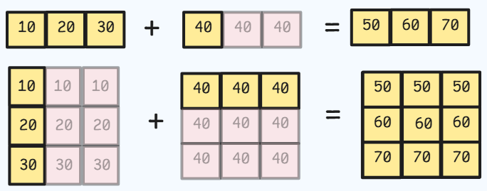
Broadcasting

It describes a set of rules on how to perform element-wise operations on tensors of different, but compatible, shapes without without explicitly copying data.
It is done automatically by libraries like PyTorch for operations like addition, subtraction, multiplication, etc.
Broadcasting follows 2 rules which are checked from right-most (trailing) dimension to left-most (leading) dimension.
1. Align Dimension
  - If the 2 tensors have different number of dimensions, the smaller tensor is padded with dimensions of size 1 on its left until both tensors have equal number of dimensions.
2. Check Dimension Compatibility
  - Now that both tensors have same number of dimensions, for each dimension the one of the following must be true :
    - The dimensions are equal.
    - One of the dimensions is 1.

If both rules are satified for all dimensions then the tensors are broadcast-compatible.

PyTorch will virtually stretch (or repeat) the smaller tensor along any dimension where its size is 1 to match the larger tensor.

No actual data is copied and unnecessary data duplication is avoided.

How is it done in MHA-Masking :

attn_scores is of shape : [batch_size, num_heads, seq_len, seq_len].
- eg. [32, 8, 50, 50]
mask is of shape : [seq_len, seq_len]
- eg. [50, 50]

1. Write down the shapes aligned to right :

attn_score : [32, 8, 50, 50]
mask : [ , , 50, 50]

2. Apply rule 1 (aligning the dimensions) :

attn_score : [32, 8, 50, 50]
mask : [ 1, 1, 50, 50]

3. Apply rule 2 (check compatibility) :

dim(-1) : 50 = 50. Thus they are equal.
dim(-2) : 50 = 50. Thus they are equal.
dim(-3) : One of them is 1.
dim(-4) : One of them is 1.
Thus, both the vectors are compatible.
Now, the tensor of shape [1, 1, 50, 50] is stretched along dim(-3) to the shape : [1, 8, 50, 50].
The resultant tensor is stretched along dim(-4) to the shape of the attn_score : [32, 8, 50, 50 ]

7. Types of MHA Used

In transformer architecture, there are 3 ways in which Multi-Head Attention is utilized :
1. Self Attention
2. Cross Attention
3. Masked Atention (Already covered above)

Self Attention

When the query, keys, and values all come from the same sequence / place (output of the previous layer), the mechanism is known as self-attention.
These layers are present in the Encoder block.
A word in the sentence will attend to all words / positions in the previous layer of the encoder.

Cross Attention / Encoder-Decoder Attention

It is the MHA layer of the Decoder stack, which comes just after the Masked MHA.
The Queries come from the previous decoder layer,
The Keys and Values come from the output of the encoder.
This allows the model to attend to all the positions in the previous layer of the encoder.

8. Embedding & Positional Encoding

Embeddings

There are 2 Embedding layers : a. Convert input tokens to vectors b. Convert target tokens to vectors
Both these layers share their weight matrix.
They also share their weight with the final linear layer that transforms the decoder’s hidden states into logits over the vocabulary before applying softmax.

Each token is mapped to a vector via the embedding matrix $ E \in \mathbb{R}^{V \times d_{model}} $.

$V$ is the vocabulary size.

It is the total number of unique tokens in the vocabulary.

When the $i^{th}$ token comes, the $i^{th}$ row is looked in $E$.

This vector / row of size $d_{model}$ is the embedding vector of that token.

This vector is scaled by $ d_{model} $ through element-wise multiplication.

It is done to normalize variance.

Positional Encoding

Need of Positional Encoding (PE) :

Transformers don’t have any notion of sequence order.
They process all tokens in parallel.
Thus, the model needs a way to know which word comes before or after another word.

Requirements

Positional Encodings must be same for a position irresepective of the sequence lenghts or the input sequnce.

They must not be too large else they may push the embedding vectors in such a way that their semantic similarity may change.

Working of PE :

The method used in the paper used fixed non-trainable PE. Newer models used learnable PE.

Use sine and cosie functions of different frequencies to encode positions.
PE can be thought of as an address vector of each token in the sequence.

Positional Encoding vector is added and not concatenated to the Embedding vector.

Waves are used to create the address vectors.

\[PE_{(pos,2i)} = \sin\left( \frac{pos}{10000^{\frac{2i}{d_{model}}}} \right)\] \[PE_{(pos,2i+1)} = \cos\left( \frac{pos}{10000^{\frac{2i}{d_{model}}}} \right)\]

$pos$ : position of the token in the sentence.
$i$ : dimension index of the embedding vector.
- i = 0 is the first dimension.
- …
- i = 255 is the last dimension. (if $d_{model} = 512$)
$i$ can be thought of as an index of for a pair of dimensions.

Analogy

A clock has 3 hands each moving at a different frequency.

Each hands gives more information about what the time is.

Same logic is being applied here, each dimension of each embedded vector at position “pos” forms a different argument or frequency for the sine / cosine functions.

For a token at a specific position pos, a Positional Encoding (PE) vector of the same dimension as the token embedding (d_model) is created.
The entries of this PE vector are found as follows:
1. An iterator, let’s call it $i$, runs from 0 to d_model / 2 - 1.
2. For each value of $i$, a unique frequency is defines.
3. This frequency is used to create one pair of waves: a sine wave and a cosine wave.
4. The sine wave’s value is placed in dimension 2i of the vector, and the cosine wave’s value is placed in dimension 2i+1.
5. For a given position pos, its corresponding point on each of these d_model total waves is calculated.
6. These d_model points form the entries of the final PE vector for that position pos.

Example

d_model = 6. Thus, $i$ goes from 0 to 2 (6/2 -1).
Thus there are 3 frequency pairs each consisting of a sine and a cosine wave.

Visualizing Positional Encoding

def pe(max_seq_len, d_model):
    pe = np.zeros((max_seq_len, d_model))
    pos = np.arrange(0, max_seq_len, dtype=np.float32).reshape(-1,1)

    div_term = np.exp(np.arrange(0, d_model, 2).astype(np.float32) * -(np.log(10000.0) / d_model))

    # Apply sin to even indices (2i)
    pe[:, 0::2] = np.sin(position * div_term)

    # Apply cos to odd indices (2i + 1)
    pe[:, 1::2] = np.cos(position * div_term)
    
    return pe
max_seq_len = 100
d_model = 128
pe_matrix = pe(max_seq_len, d_model)

Practical Implementation

In the above code the numpy line : div_term = np.exp(np.arrange(0, d_model, 2).astype(np.float32) * -(np.log(10000.0) / d_model)) is written in PyTorch like :

div_term = torch.exp(torch.arange(0, d_model, 2).float() * (-math.log(10000.0) / d_model)) # (d_model / 2)

The denominator in the paper is :

\[10000^{\frac{2i}{d_{model}}}\]

It is same as :

\[\exp\left ( -\ln{(10000)} \cdot \frac{2i}{d_{model}} \right )\]

Using exp and log is more stable for floating point calculations for very large or small numbers.
torch.exp() is vectorized and optimized.

Detailed Flow of Information in Transformer

Now that all the major parts of the transformer are covered, it’s time to see how information flows through the transformer. This is going to be a high level description of the first diagram.

Encoder

Sentences are encoded using Byte Pair Encoding (BPE).
- In this algorithm, most frequent pairs of bytes (chars) are iteratively merged to form larger units.
The encoded token sequences of similar length are grouped in batchesto avoid wasting computation on padding tokens for shorted sentences.
Once encoded, the Positional Encoding is added to the Embedding matrix.
Now the tokens are fed into the the main encoder block.
Multi Head Self Attention is performed on the input.
After this the output from the MHA layer as well as the original input are added via the skip connections and layer normalization is performed.
- Skip connection help in maintaining the positional encoding through the models depth.
Then the information flows through a Position Wise Feed Forward NN and agian the input and the out of this layer are added and layer normalization is performed.

Now the encoders can be stacked, where output from one encoder becomes the input of the next encoder.

Decoder

During Training

Teacher Forcing Method is used during training where the entire ground truth output sequence is fed to the decoder at once.
Ground truth values added with the positional encoding are fed into Masked Multi-Head Self Attention and the output is a sequence where each token has attended to the preceding tokens.
This output is used to generate the Query vectors the next sub-layer Encoder-Decoder Attention.
The Key and Value for this layer comes from the Enocoder’s output.
The output from the cross attention layer is fed into the Feed-Forward Layer.
The final output is passed through a linear layer and then a softmax function to produce a probability distribution over the entire vocabulary for each position in the output sequence.

The loss is then calculated by comparing these predicted probabilities with the actual next tokens in the ground-truth sequence.

During Inference (Auto-Regressive)

The decoder’s first input is the start token <sos>. It is converted to into an embedding and PE is added to it.
It is the input to the the Masked Muti Head Self Attention.
The output acts as the query and it attends to the keys and values vectors from the encoder.
Then same as in training phase the output is passed through the FFN and then a linear layer follwed by softmax prediction.
The predicted token is then appended to the exisiting sequence of generated sequence.
This new sequence then becomes the input to masked MHA layer in the next step.
This process is continued till the final end of sequence token <eos> is not generated.

Attention Is All You Need Deep Dive

1. Background

2. Transformer Architecture Overview

Encoder

Residual Connection

Layer Norm

Internal Covariate Shift

Mean :

Variance :

Normalize :

Scale & Shift :

Decoder

3. Position-wise fully connected feed-forward network

4. Scaled Dot Product Attention

Mathematical formulation of Scaled Dot Product Attention

a. Dot Product

b. Scaling

c. Applying Softmax

d. Multiply with Values

5. Multi-Head Attention

The Conceptual Model :

The Practical Implementation :

The Conceptual Model

1. Initial Generation of Master Q,K,V :

2. Split : [Head-specific Projections]

3. Parallel Attention Calculation

4. Concatenation and Final Projection

The Practical Implementation

1. Fusing the projection steps

2. Reshape and Transpose for Heads [Split part]

3. Batch Scaled Dot-Product Attention Calculation

4. Reverse, Reshape and Final Projection (Concatenation):

6. Masked Multi-Head Attention

1. Create a Mask Matrix :

2. Apply the mask to scaled scores :

3. Working of the Mask :

4. Implementation using Multi-Heads :

Broadcasting

How is it done in MHA-Masking :

1. Write down the shapes aligned to right :

2. Apply rule 1 (aligning the dimensions) :

3. Apply rule 2 (check compatibility) :

7. Types of MHA Used

Self Attention

Cross Attention / Encoder-Decoder Attention

8. Embedding & Positional Encoding

Embeddings

Positional Encoding

Need of Positional Encoding (PE) :

Working of PE :

Example

Visualizing Positional Encoding

Practical Implementation

Detailed Flow of Information in Transformer

Encoder

Decoder

During Training

During Inference (Auto-Regressive)

References